Aquaponics System Balance

Summary

This experiment investigates aquaponics system balance. Box-Behnken design to maximize fish growth and plant yield by tuning fish density, feeding rate, and water flow rate.

The design varies 3 factors: fish density (fish/m3), ranging from 10 to 40, feed rate pct (%BW/day), ranging from 1 to 4, and flow rate lph (L/hr), ranging from 200 to 800. The goal is to optimize 2 responses: fish growth g (g/week) (maximize) and plant yield g (g/m2/wk) (maximize). Fixed conditions held constant across all runs include fish species = tilapia, plant = basil.

A Box-Behnken design was chosen because it efficiently fits quadratic models with 3 continuous factors while avoiding extreme corner combinations — requiring only 15 runs instead of the 8 needed for a full factorial at two levels.

Quadratic response surface models were fitted to capture potential curvature and factor interactions. The RSM contour plots below visualize how pairs of factors jointly affect each response.

Key Findings

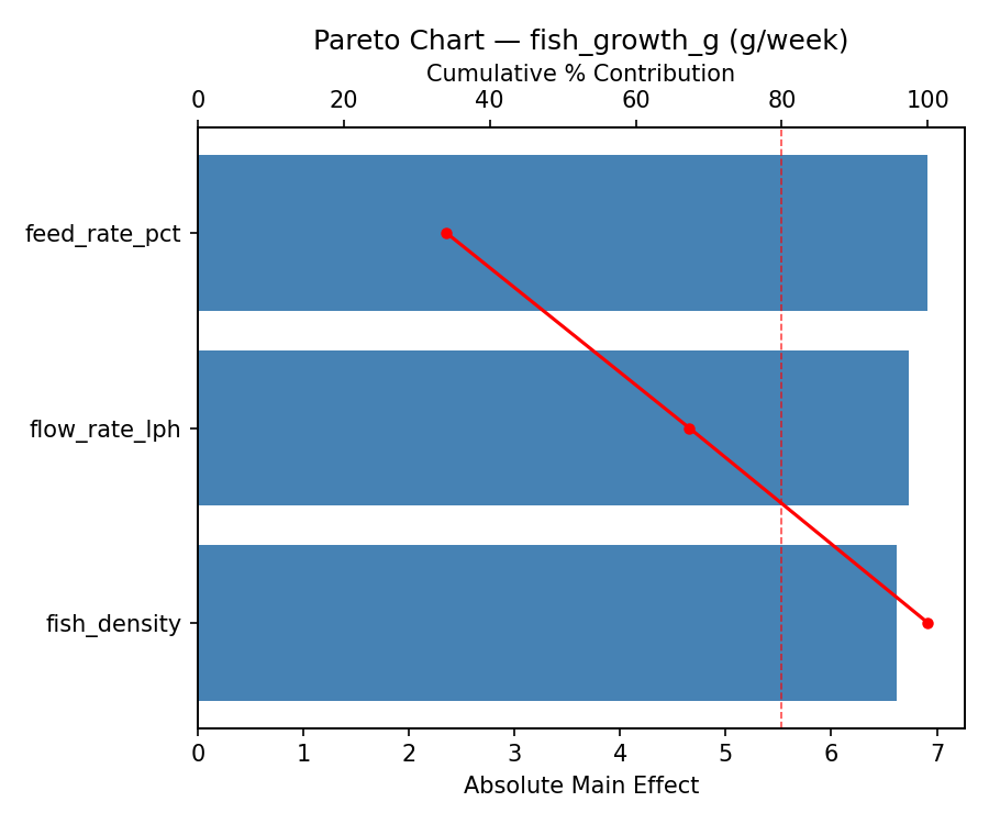
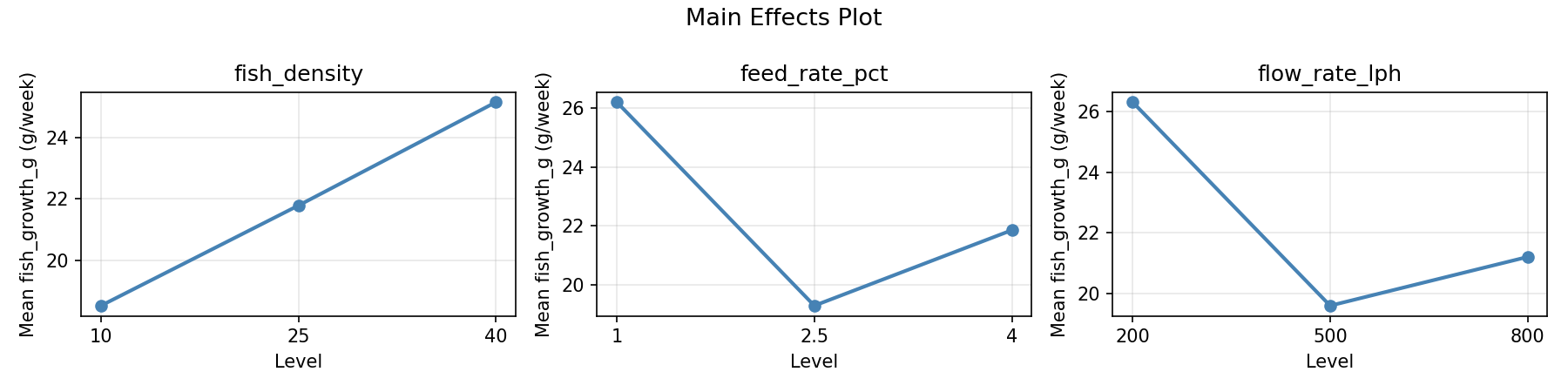
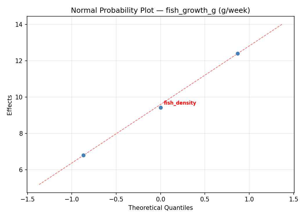
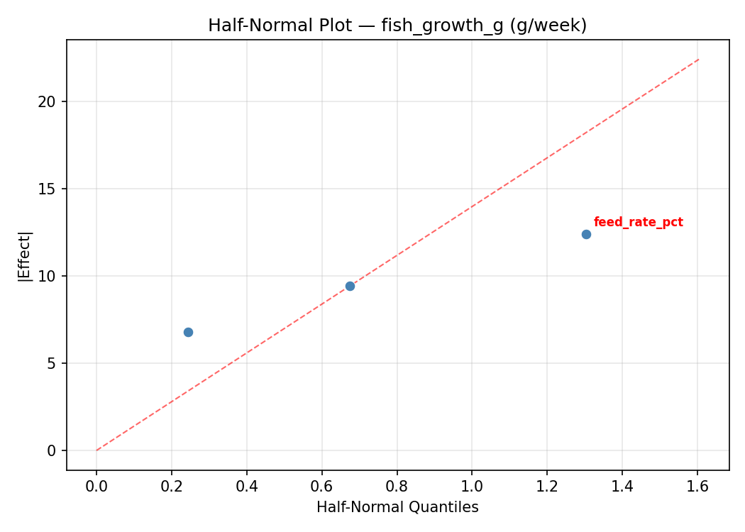
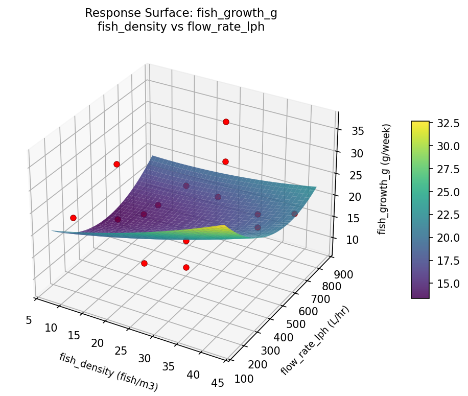
For fish growth g, the most influential factors were flow rate lph (45.2%), fish density (33.0%), feed rate pct (21.8%). The best observed value was 36.7 (at fish density = 25, feed rate pct = 2.5, flow rate lph = 500).

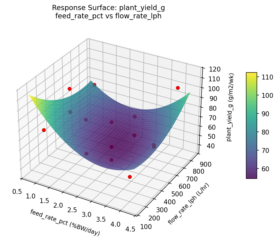
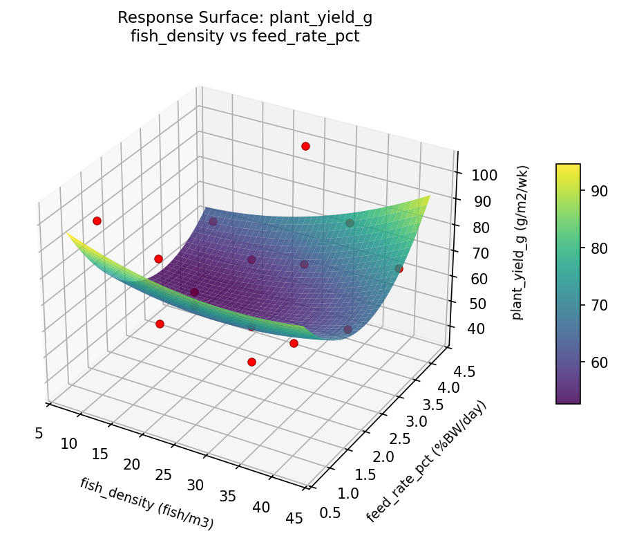
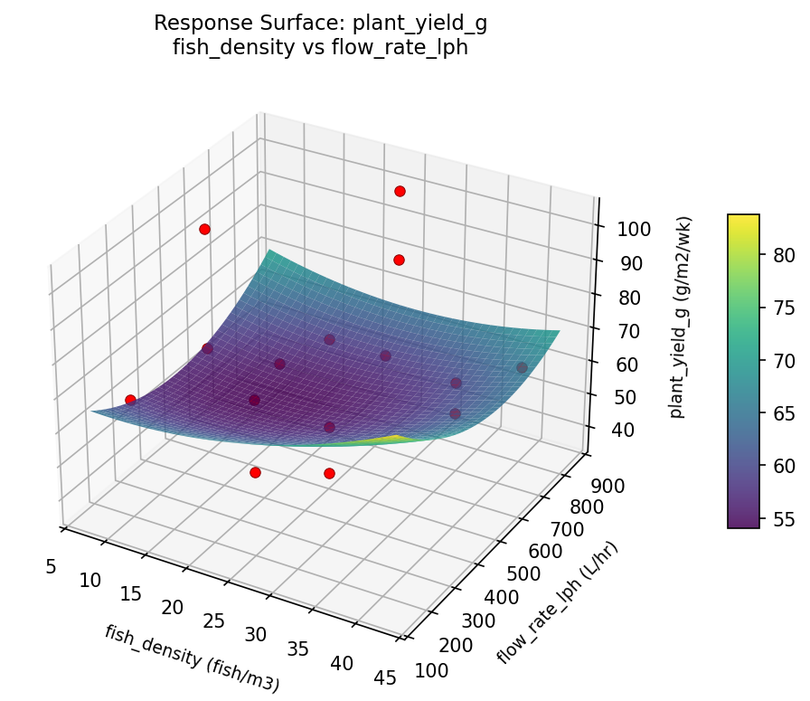
For plant yield g, the most influential factors were flow rate lph (40.8%), fish density (31.2%), feed rate pct (28.1%). The best observed value was 103.0 (at fish density = 25, feed rate pct = 2.5, flow rate lph = 500).

Recommended Next Steps

Run confirmation experiments at the predicted optimal settings to validate the model.
Consider whether any fixed factors should be varied in a future study.

Experimental Setup

Factors

Factor	Low	High	Unit
`fish_density`	10	40	fish/m3
`feed_rate_pct`	1	4	%BW/day
`flow_rate_lph`	200	800	L/hr

Fixed: fish_species = tilapia, plant = basil

Responses

Response	Direction	Unit
`fish_growth_g`	↑ maximize	g/week
`plant_yield_g`	↑ maximize	g/m2/wk

Configuration

use_cases/135_aquaponics_balance/config.json

{
  "metadata": {
    "name": "Aquaponics System Balance",
    "description": "Box-Behnken design to maximize fish growth and plant yield by tuning fish density, feeding rate, and water flow rate"
  },
  "factors": [
    {
      "name": "fish_density",
      "levels": [
        "10",
        "40"
      ],
      "type": "continuous",
      "unit": "fish/m3"
    },
    {
      "name": "feed_rate_pct",
      "levels": [
        "1",
        "4"
      ],
      "type": "continuous",
      "unit": "%BW/day"
    },
    {
      "name": "flow_rate_lph",
      "levels": [
        "200",
        "800"
      ],
      "type": "continuous",
      "unit": "L/hr"
    }
  ],
  "fixed_factors": {
    "fish_species": "tilapia",
    "plant": "basil"
  },
  "responses": [
    {
      "name": "fish_growth_g",
      "optimize": "maximize",
      "unit": "g/week"
    },
    {
      "name": "plant_yield_g",
      "optimize": "maximize",
      "unit": "g/m2/wk"
    }
  ],
  "settings": {
    "operation": "box_behnken",
    "test_script": "use_cases/135_aquaponics_balance/sim.sh"
  }
}

Experimental Matrix

The Box-Behnken Design produces 15 runs. Each row is one experiment with specific factor settings.

Run	`fish_density`	`feed_rate_pct`	`flow_rate_lph`
1	25	1	200
2	25	2.5	500
3	40	2.5	800
4	40	2.5	200
5	25	2.5	500
6	25	2.5	500
7	10	2.5	800
8	40	1	500
9	25	1	800
10	40	4	500
11	10	2.5	200
12	25	4	800
13	10	1	500
14	10	4	500
15	25	4	200

Step-by-Step Workflow

1

Preview the design

Terminal

$ doe info --config use_cases/135_aquaponics_balance/config.json

2

Generate the runner script

Terminal

$ doe generate --config use_cases/135_aquaponics_balance/config.json \
    --output use_cases/135_aquaponics_balance/results/run.sh --seed 42

3

Execute the experiments

Terminal

$ bash use_cases/135_aquaponics_balance/results/run.sh

4

Analyze results

Terminal

$ doe analyze --config use_cases/135_aquaponics_balance/config.json

5

Get optimization recommendations

Terminal

$ doe optimize --config use_cases/135_aquaponics_balance/config.json

6

Multi-objective optimization

With 2 competing responses, use --multi to find the best compromise via Derringer–Suich desirability.

Terminal

$ doe optimize --config use_cases/135_aquaponics_balance/config.json --multi

7

Generate the HTML report

Terminal

$ doe report --config use_cases/135_aquaponics_balance/config.json \
    --output use_cases/135_aquaponics_balance/results/report.html

Features Exercised

Feature	Value
Design type	`box_behnken`
Factor types	`continuous` (all 3)
Arg style	`double-dash`
Responses	2 (fish_growth_g ↑, plant_yield_g ↑)
Total runs	15

Analysis Results

Generated from actual experiment runs using the DOE Helper Tool.

Response: fish_growth_g

Top factors: flow_rate_lph (45.2%), fish_density (33.0%), feed_rate_pct (21.8%).

ANOVA

Source	DF	SS	MS	F	p-value
Source	DF	SS	MS	F	p-value
fish_density	2	145.3480	72.6740	24.442	0.0004
feed_rate_pct	2	63.7902	31.8951	10.727	0.0054
flow_rate_lph	2	376.8130	188.4065	63.365	0.0000
Lack	of	Fit	6	377.9194	62.9866
Pure	Error	2	5.9467
Error	8	383.8660	2.9733
Total	14	969.8173	69.2727

Pareto Chart

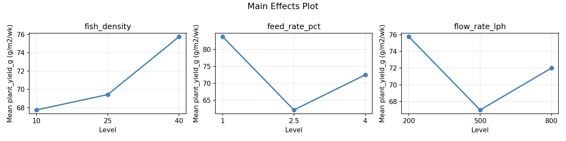
Main Effects Plot

Normal Probability Plot of Effects

Normal probability plot for fish_growth_g

Half-Normal Plot of Effects

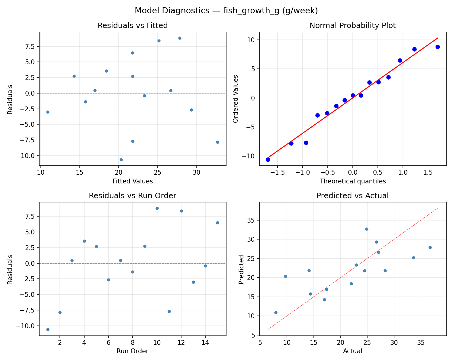
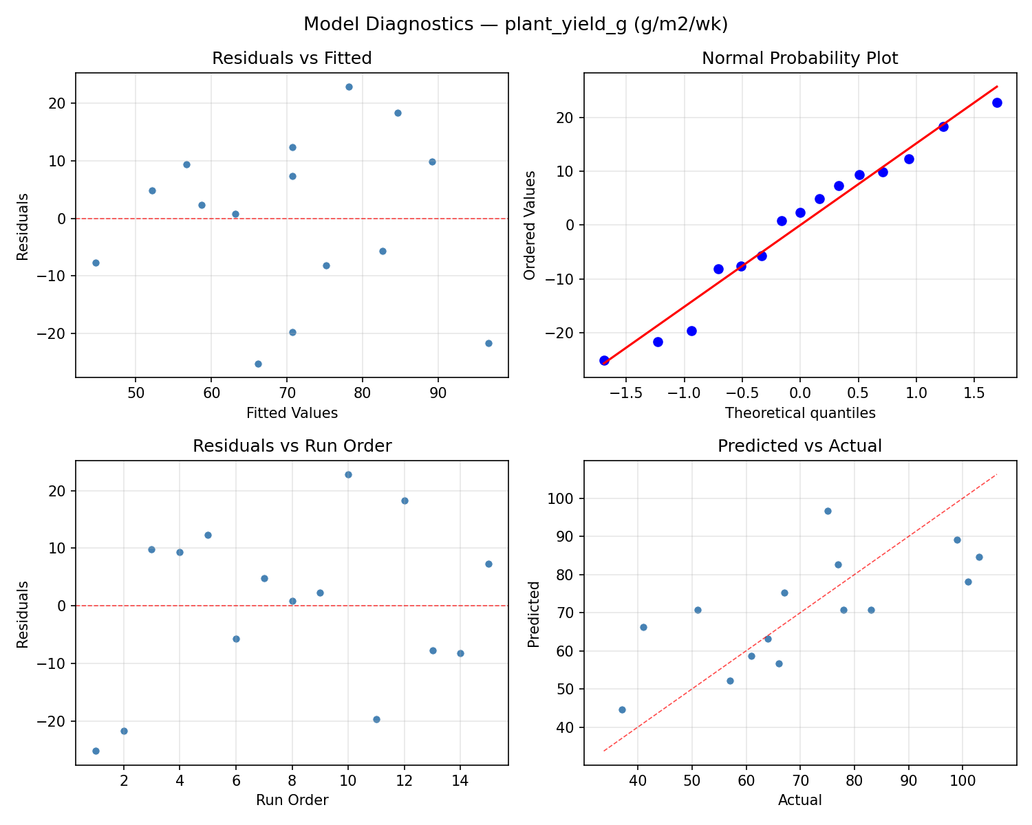
Model Diagnostics

Response: plant_yield_g

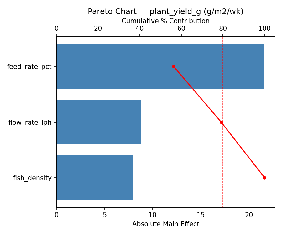
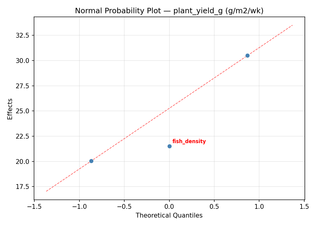
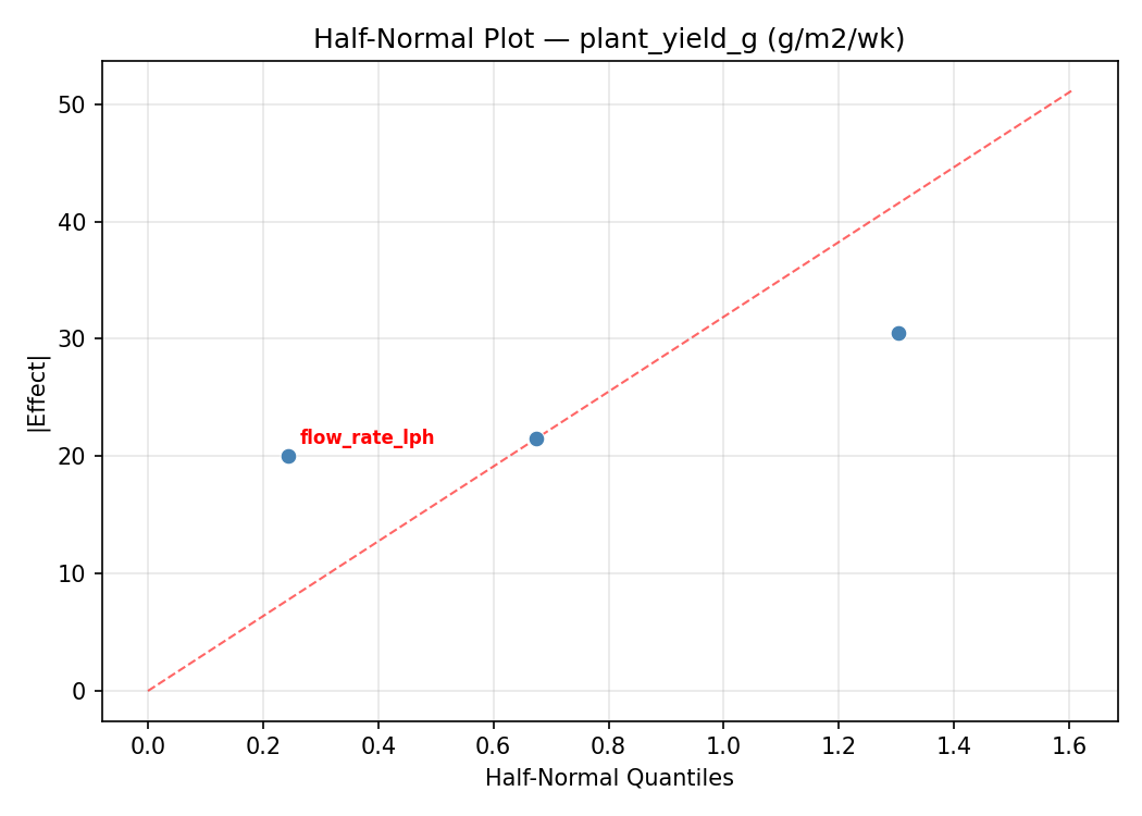
Top factors: flow_rate_lph (40.8%), fish_density (31.2%), feed_rate_pct (28.1%).

ANOVA

Source	DF	SS	MS	F	p-value
Source	DF	SS	MS	F	p-value
fish_density	2	780.1548	390.0774	2.281	0.1645
feed_rate_pct	2	612.1190	306.0595	1.790	0.2278
flow_rate_lph	2	1908.1548	954.0774	5.579	0.0304
Lack	of	Fit	6	2150.9048	358.4841
Pure	Error	2	342.0000
Error	8	2492.9048	171.0000
Total	14	5793.3333	413.8095

Pareto Chart

Main Effects Plot

Normal Probability Plot of Effects

Normal probability plot for plant_yield_g

Half-Normal Plot of Effects

Model Diagnostics

Response Surface Plots

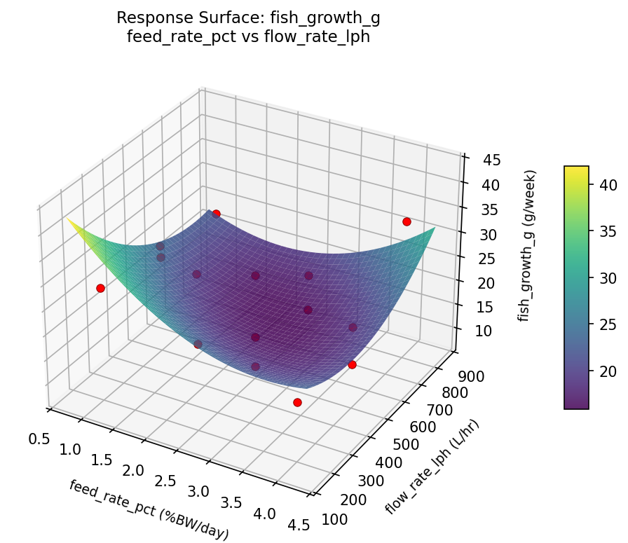
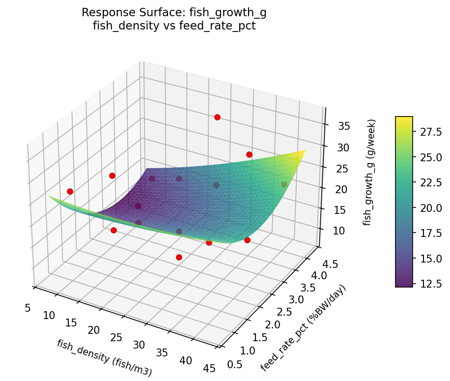
3D surfaces fitted with quadratic RSM. Red dots are observed data points.

fish growth g feed rate pct vs flow rate lph

fish growth g fish density vs feed rate pct

fish growth g fish density vs flow rate lph

plant yield g feed rate pct vs flow rate lph

plant yield g fish density vs feed rate pct

plant yield g fish density vs flow rate lph

Multi-Objective Optimization

When responses compete, Derringer–Suich desirability finds the best compromise. Each response is scaled to a 0–1 desirability, then combined via a weighted geometric mean.

Overall Desirability

D = 1.0000

Per-Response Desirability

Response	Weight	Desirability	Predicted	Dir
`fish_growth_g`	1.5	1.0000	38.52 1.0000 38.52 g/week	↑
`plant_yield_g`	1.5	1.0000	115.29 1.0000 115.29 g/m2/wk	↑

Recommended Settings

Factor	Value
`fish_density`	10 fish/m3
`feed_rate_pct`	1 %BW/day
`flow_rate_lph`	200 L/hr

Source: from RSM model prediction

Trade-off Summary

Sacrifice = how much worse than single-objective best.

Response	Predicted	Best Observed	Sacrifice
`plant_yield_g`	115.29	103.00	-12.29

Top 3 Runs by Desirability

Run	D	Factor Settings
#12	0.9043	fish_density=10, feed_rate_pct=1, flow_rate_lph=500
#3	0.7655	fish_density=40, feed_rate_pct=2.5, flow_rate_lph=800

Model Quality

Response	R²	Type
`plant_yield_g`	0.8272	quadratic

Full Multi-Objective Output

doe optimize --multi
============================================================
MULTI-OBJECTIVE OPTIMIZATION
Method: Derringer-Suich Desirability Function
============================================================

Overall desirability: D = 1.0000

Response                  Weight Desirability    Predicted  Direction
---------------------------------------------------------------------
fish_growth_g                1.5       1.0000       38.52 g/week   ↑
plant_yield_g                1.5       1.0000      115.29 g/m2/wk   ↑

Recommended settings:
  fish_density = 10 fish/m3
  feed_rate_pct = 1 %BW/day
  flow_rate_lph = 200 L/hr
  (from RSM model prediction)

Trade-off summary:
  fish_growth_g: 38.52 (best observed: 36.70, sacrifice: -1.82)
  plant_yield_g: 115.29 (best observed: 103.00, sacrifice: -12.29)

Model quality:
  fish_growth_g: R² = 0.8106 (quadratic)
  plant_yield_g: R² = 0.8272 (quadratic)

Top 3 observed runs by overall desirability:
  1. Run #10 (D=0.9407): fish_density=40, feed_rate_pct=4, flow_rate_lph=500
  2. Run #12 (D=0.9043): fish_density=10, feed_rate_pct=1, flow_rate_lph=500
  3. Run #3 (D=0.7655): fish_density=40, feed_rate_pct=2.5, flow_rate_lph=800

Full Analysis Output

doe analyze
=== Main Effects: fish_growth_g ===
Factor                   Effect    Std Error   % Contribution
--------------------------------------------------------------
flow_rate_lph           10.0714       2.1490            45.2%
fish_density             7.3536       2.1490            33.0%
feed_rate_pct            4.8500       2.1490            21.8%

=== ANOVA Table: fish_growth_g ===
Source                      DF           SS           MS          F    p-value
-----------------------------------------------------------------------------
fish_density                 2     145.3480      72.6740     24.442     0.0004
feed_rate_pct                2      63.7902      31.8951     10.727     0.0054
flow_rate_lph                2     376.8130     188.4065     63.365     0.0000
Lack of Fit                  6     377.9194      62.9866     21.184     0.0458
Pure Error                   2       5.9467       2.9733
Error                        8     383.8660       2.9733
Total                       14     969.8173      69.2727

=== Summary Statistics: fish_growth_g ===

fish_density:
  Level               N       Mean        Std        Min        Max
  ------------------------------------------------------------
  10                  4    20.6250    11.8635     9.7000    36.7000
  25                  7    19.5714     7.4783     7.9000    28.3000
  40                  4    26.9250     4.7148    22.9000    33.6000

feed_rate_pct:
  Level               N       Mean        Std        Min        Max
  ------------------------------------------------------------
  1                   4    23.2500     9.9165    14.4000    36.7000
  2.5                 7    22.9429     8.3362     9.7000    33.6000
  4                   4    18.4000     8.0428     7.9000    26.7000

flow_rate_lph:
  Level               N       Mean        Std        Min        Max
  ------------------------------------------------------------
  200                 4    17.1000     4.0800    14.1000    22.9000
  500                 7    27.1714     4.6786    22.0000    36.7000
  800                 4    17.1500    11.7151     7.9000    33.6000

=== Main Effects: plant_yield_g ===
Factor                   Effect    Std Error   % Contribution
--------------------------------------------------------------
flow_rate_lph           23.2143       5.2524            40.8%
fish_density            17.7500       5.2524            31.2%
feed_rate_pct           16.0000       5.2524            28.1%

=== ANOVA Table: plant_yield_g ===
Source                      DF           SS           MS          F    p-value
-----------------------------------------------------------------------------
fish_density                 2     780.1548     390.0774      2.281     0.1645
feed_rate_pct                2     612.1190     306.0595      1.790     0.2278
flow_rate_lph                2    1908.1548     954.0774      5.579     0.0304
Lack of Fit                  6    2150.9048     358.4841      2.096     0.3577
Pure Error                   2     342.0000     171.0000
Error                        8    2492.9048     171.0000
Total                       14    5793.3333     413.8095

=== Summary Statistics: plant_yield_g ===

fish_density:
  Level               N       Mean        Std        Min        Max
  ------------------------------------------------------------
  10                  4    64.7500    26.2599    41.0000   101.0000
  25                  7    67.2857    19.3797    37.0000    99.0000
  40                  4    82.5000    15.1767    67.0000   103.0000

feed_rate_pct:
  Level               N       Mean        Std        Min        Max
  ------------------------------------------------------------
  1                   4    76.2500    19.8221    57.0000   101.0000
  2.5                 7    73.4286    22.9046    41.0000   103.0000
  4                   4    60.2500    16.8795    37.0000    77.0000

flow_rate_lph:
  Level               N       Mean        Std        Min        Max
  ------------------------------------------------------------
  200                 4    60.7500     6.9462    51.0000    67.0000
  500                 7    82.7143    12.8675    66.0000   101.0000
  800                 4    59.5000    30.2600    37.0000   103.0000

Optimization Recommendations

doe optimize
=== Optimization: fish_growth_g ===
Direction: maximize

Best observed run: #10
  fish_density = 25
  feed_rate_pct = 2.5
  flow_rate_lph = 500
  Value: 36.7

RSM Model (linear, R² = 0.3030, Adj R² = 0.1129):
  Coefficients:
    intercept                      +21.8133
    fish_density                   -4.2125
    feed_rate_pct                  +0.9625
    flow_rate_lph                  +4.2500

RSM Model (quadratic, R² = 0.5792, Adj R² = -0.1781):
  Coefficients:
    intercept                      +29.1000
    fish_density                   -4.2125
    feed_rate_pct                  +0.9625
    flow_rate_lph                  +4.2500
    fish_density*feed_rate_pct     +1.5250
    fish_density*flow_rate_lph     +1.8000
    feed_rate_pct*flow_rate_lph    -1.4000
    fish_density^2                 -2.1625
    feed_rate_pct^2                -5.0125
    flow_rate_lph^2                -6.4875

  Curvature analysis:
    flow_rate_lph                  coef=-6.4875  concave (has a maximum)
    feed_rate_pct                  coef=-5.0125  concave (has a maximum)
    fish_density                   coef=-2.1625  concave (has a maximum)

  Notable interactions:
    fish_density*flow_rate_lph     coef=+1.8000  (synergistic)
    fish_density*feed_rate_pct     coef=+1.5250  (synergistic)
    feed_rate_pct*flow_rate_lph    coef=-1.4000  (antagonistic)

  Predicted optimum (from linear model, at observed points):
    fish_density = 10
    feed_rate_pct = 2.5
    flow_rate_lph = 800
    Predicted value: 30.2758

  Surface optimum (via L-BFGS-B, linear model):
    fish_density = 10
    feed_rate_pct = 4
    flow_rate_lph = 800
    Predicted value: 31.2383

  Model quality: Weak fit — consider adding center points or using a different design.

Factor importance:
  1. flow_rate_lph  (effect: 10.2, contribution: 42.6%)
  2. fish_density  (effect: 8.4, contribution: 35.1%)
  3. feed_rate_pct  (effect: 5.4, contribution: 22.3%)

=== Optimization: plant_yield_g ===
Direction: maximize

Best observed run: #12
  fish_density = 25
  feed_rate_pct = 2.5
  flow_rate_lph = 500
  Value: 103.0

RSM Model (linear, R² = 0.1944, Adj R² = -0.0252):
  Coefficients:
    intercept                      +70.6667
    fish_density                   -10.0000
    feed_rate_pct                  +3.2500
    flow_rate_lph                  +5.5000

RSM Model (quadratic, R² = 0.4815, Adj R² = -0.4517):
  Coefficients:
    intercept                      +88.3333
    fish_density                   -10.0000
    feed_rate_pct                  +3.2500
    flow_rate_lph                  +5.5000
    fish_density*feed_rate_pct     +3.2500
    fish_density*flow_rate_lph     +6.2500
    feed_rate_pct*flow_rate_lph    +0.2500
    fish_density^2                 -4.5417
    feed_rate_pct^2                -16.5417
    flow_rate_lph^2                -12.0417

  Curvature analysis:
    feed_rate_pct                  coef=-16.5417  concave (has a maximum)
    flow_rate_lph                  coef=-12.0417  concave (has a maximum)
    fish_density                   coef=-4.5417  concave (has a maximum)

  Notable interactions:
    fish_density*flow_rate_lph     coef=+6.2500  (synergistic)
    fish_density*feed_rate_pct     coef=+3.2500  (synergistic)

  Predicted optimum (from linear model, at observed points):
    fish_density = 10
    feed_rate_pct = 2.5
    flow_rate_lph = 800
    Predicted value: 86.1667

  Surface optimum (via L-BFGS-B, linear model):
    fish_density = 10
    feed_rate_pct = 4
    flow_rate_lph = 800
    Predicted value: 89.4167

  Model quality: Weak fit — consider adding center points or using a different design.

Factor importance:
  1. fish_density  (effect: 20.0, contribution: 36.6%)
  2. feed_rate_pct  (effect: 18.6, contribution: 34.1%)
  3. flow_rate_lph  (effect: 16.0, contribution: 29.3%)

Run	`fish_density`	`feed_rate_pct`	`flow_rate_lph`
1	25	1	200
2	25	2.5	500
3	40	2.5	800
4	40	2.5	200
5	25	2.5	500
6	25	2.5	500
7	10	2.5	800
8	40	1	500
9	25	1	800
10	40	4	500
11	10	2.5	200
12	25	4	800
13	10	1	500
14	10	4	500
15	25	4	200

Run	`fish_density`	`feed_rate_pct`	`flow_rate_lph`
1	25	1	200
2	25	2.5	500
3	40	2.5	800
4	40	2.5	200
5	25	2.5	500
6	25	2.5	500
7	10	2.5	800
8	40	1	500
9	25	1	800
10	40	4	500
11	10	2.5	200
12	25	4	800
13	10	1	500
14	10	4	500
15	25	4	200

Run	`fish_density`	`feed_rate_pct`	`flow_rate_lph`
1	25	1	200
2	25	2.5	500
3	40	2.5	800
4	40	2.5	200
5	25	2.5	500
6	25	2.5	500
7	10	2.5	800
8	40	1	500
9	25	1	800
10	40	4	500
11	10	2.5	200
12	25	4	800
13	10	1	500
14	10	4	500
15	25	4	200