Microscope Imaging Quality

Summary

This experiment investigates microscope imaging quality. Central composite design to maximize resolution and minimize chromatic aberration by tuning objective magnification, illumination intensity, and condenser aperture.

The design varies 3 factors: magnification (x), ranging from 10 to 100, illumination pct (%), ranging from 20 to 100, and condenser na (NA), ranging from 0.2 to 0.9. The goal is to optimize 2 responses: resolution um (um) (minimize) and aberration score (pts) (minimize). Fixed conditions held constant across all runs include specimen = stained_tissue, camera = cmos_sensor.

A Central Composite Design (CCD) was selected to fit a full quadratic response surface model, including curvature and interaction effects. With 3 factors this produces 22 runs including center points and axial (star) points that extend beyond the factorial range.

Quadratic response surface models were fitted to capture potential curvature and factor interactions. The RSM contour plots below visualize how pairs of factors jointly affect each response.

Key Findings

For resolution um, the most influential factors were magnification (56.3%), illumination pct (29.2%), condenser na (14.6%). The best observed value was 1.15 (at magnification = 55, illumination pct = 60, condenser na = 0.55).

For aberration score, the most influential factors were magnification (47.1%), illumination pct (32.4%), condenser na (20.6%). The best observed value was 2.2 (at magnification = 10, illumination pct = 20, condenser na = 0.9).

Recommended Next Steps

Run confirmation experiments at the predicted optimal settings to validate the model.
Consider whether any fixed factors should be varied in a future study.

Experimental Setup

Factors

Factor	Low	High	Unit
`magnification`	10	100	x
`illumination_pct`	20	100	%
`condenser_na`	0.2	0.9	NA

Fixed: specimen = stained_tissue, camera = cmos_sensor

Responses

Response	Direction	Unit
`resolution_um`	↓ minimize	um
`aberration_score`	↓ minimize	pts

Configuration

use_cases/151_microscope_imaging/config.json

{
  "metadata": {
    "name": "Microscope Imaging Quality",
    "description": "Central composite design to maximize resolution and minimize chromatic aberration by tuning objective magnification, illumination intensity, and condenser aperture"
  },
  "factors": [
    {
      "name": "magnification",
      "levels": [
        "10",
        "100"
      ],
      "type": "continuous",
      "unit": "x"
    },
    {
      "name": "illumination_pct",
      "levels": [
        "20",
        "100"
      ],
      "type": "continuous",
      "unit": "%"
    },
    {
      "name": "condenser_na",
      "levels": [
        "0.2",
        "0.9"
      ],
      "type": "continuous",
      "unit": "NA"
    }
  ],
  "fixed_factors": {
    "specimen": "stained_tissue",
    "camera": "cmos_sensor"
  },
  "responses": [
    {
      "name": "resolution_um",
      "optimize": "minimize",
      "unit": "um"
    },
    {
      "name": "aberration_score",
      "optimize": "minimize",
      "unit": "pts"
    }
  ],
  "settings": {
    "operation": "central_composite",
    "test_script": "use_cases/151_microscope_imaging/sim.sh"
  }
}

Experimental Matrix

The Central Composite Design produces 22 runs. Each row is one experiment with specific factor settings.

Run	`magnification`	`illumination_pct`	`condenser_na`
1	55	60	0.55
2	100	20	0.9
3	10	100	0.2
4	55	133.03	0.55
5	55	60	0.55
6	-27.1584	60	0.55
7	55	60	-0.0890097
8	55	60	0.55
9	100	100	0.2
10	137.158	60	0.55
11	55	60	0.55
12	55	-13.0297	0.55
13	55	60	0.55
14	10	20	0.9
15	55	60	0.55
16	100	20	0.2
17	55	60	1.18901
18	100	100	0.9
19	55	60	0.55
20	10	20	0.2
21	10	100	0.9
22	55	60	0.55

Step-by-Step Workflow

1

Preview the design

Terminal

$ doe info --config use_cases/151_microscope_imaging/config.json

2

Generate the runner script

Terminal

$ doe generate --config use_cases/151_microscope_imaging/config.json \
    --output use_cases/151_microscope_imaging/results/run.sh --seed 42

3

Execute the experiments

Terminal

$ bash use_cases/151_microscope_imaging/results/run.sh

4

Analyze results

Terminal

$ doe analyze --config use_cases/151_microscope_imaging/config.json

5

Get optimization recommendations

Terminal

$ doe optimize --config use_cases/151_microscope_imaging/config.json

6

Multi-objective optimization

With 2 competing responses, use --multi to find the best compromise via Derringer–Suich desirability.

Terminal

$ doe optimize --config use_cases/151_microscope_imaging/config.json --multi

7

Generate the HTML report

Terminal

$ doe report --config use_cases/151_microscope_imaging/config.json \
    --output use_cases/151_microscope_imaging/results/report.html

Features Exercised

Feature	Value
Design type	`central_composite`
Factor types	`continuous` (all 3)
Arg style	`double-dash`
Responses	2 (resolution_um ↓, aberration_score ↓)
Total runs	22

Analysis Results

Generated from actual experiment runs using the DOE Helper Tool.

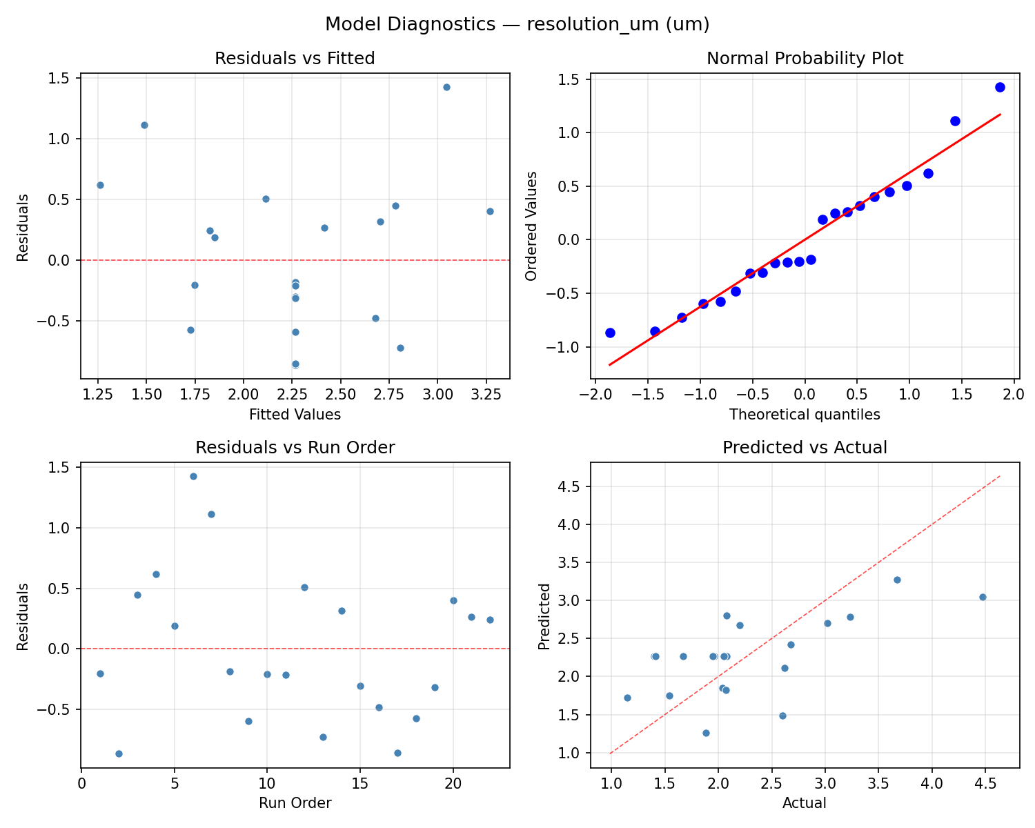
Response: resolution_um

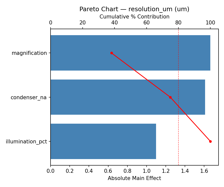
Top factors: magnification (56.3%), illumination_pct (29.2%), condenser_na (14.6%).

ANOVA

Source	DF	SS	MS	F	p-value
Source	DF	SS	MS	F	p-value
magnification	4	6.4469	1.6117	2.583	0.1092
illumination_pct	4	2.6316	0.6579	1.054	0.4322
condenser_na	4	2.0290	0.5072	0.813	0.5477
Lack	of	Fit	2	0.0000	0.0000
Pure	Error	7	4.3685
Error	9	1.8325	0.6241
Total	21	12.9399	0.6162

Pareto Chart

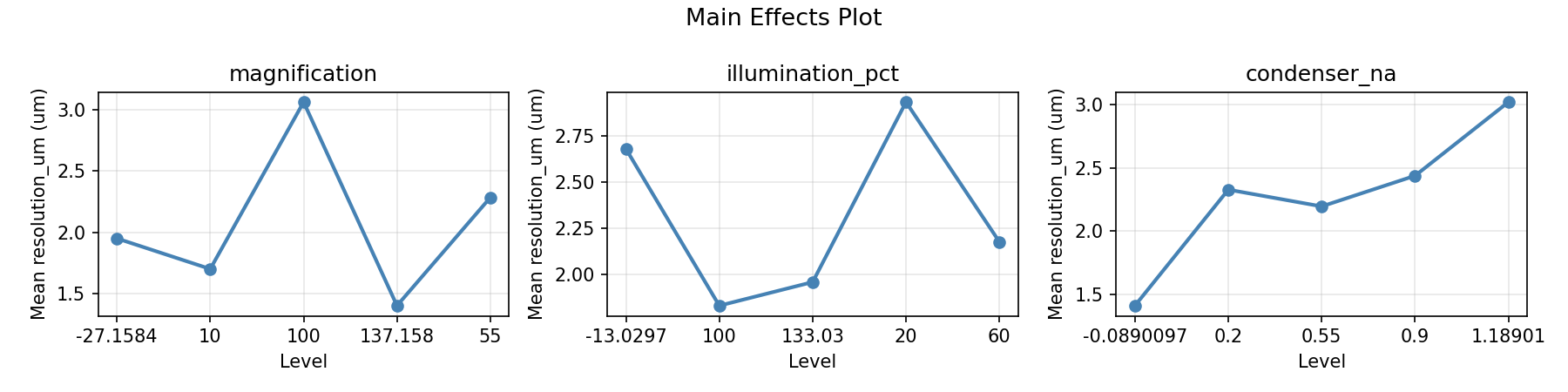
Main Effects Plot

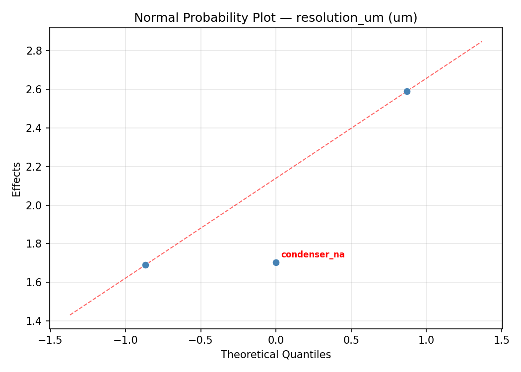
Normal Probability Plot of Effects

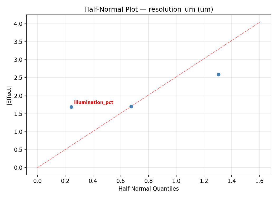
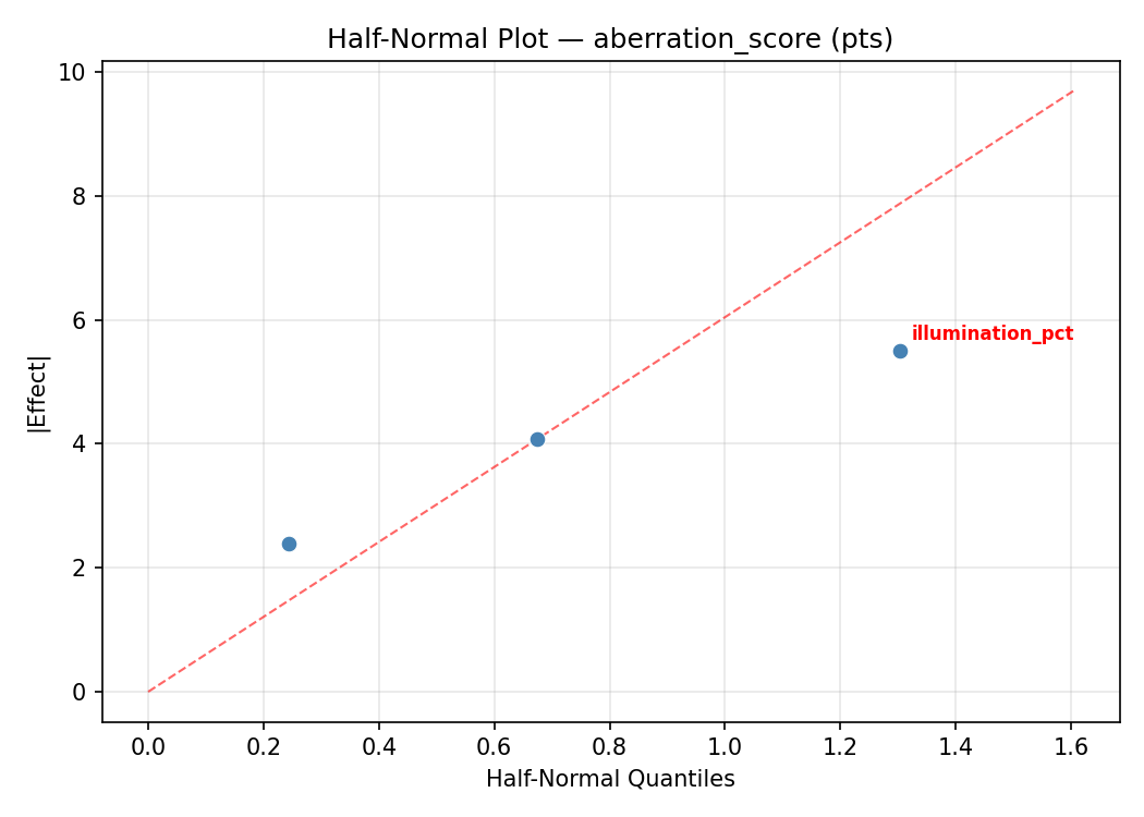
Normal probability plot for resolution_um

Half-Normal Plot of Effects

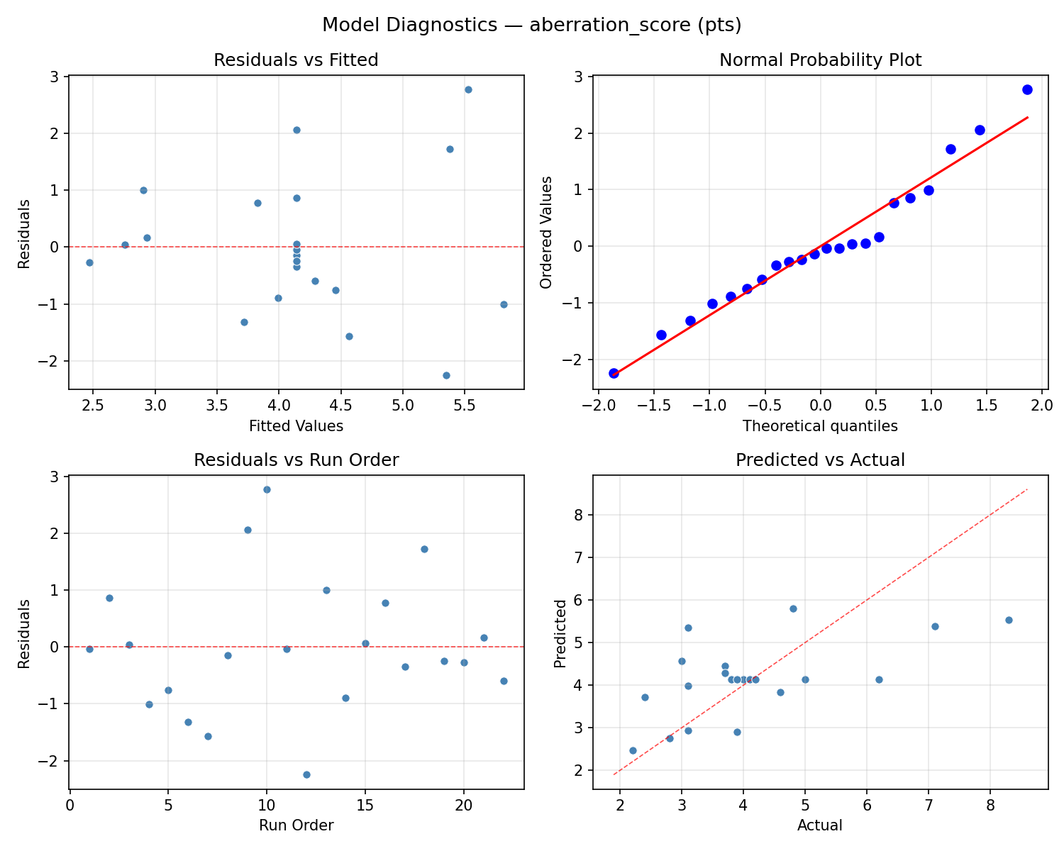
Model Diagnostics

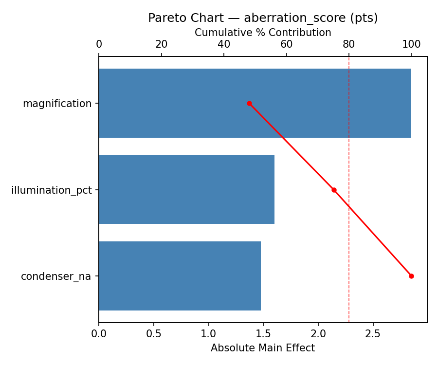
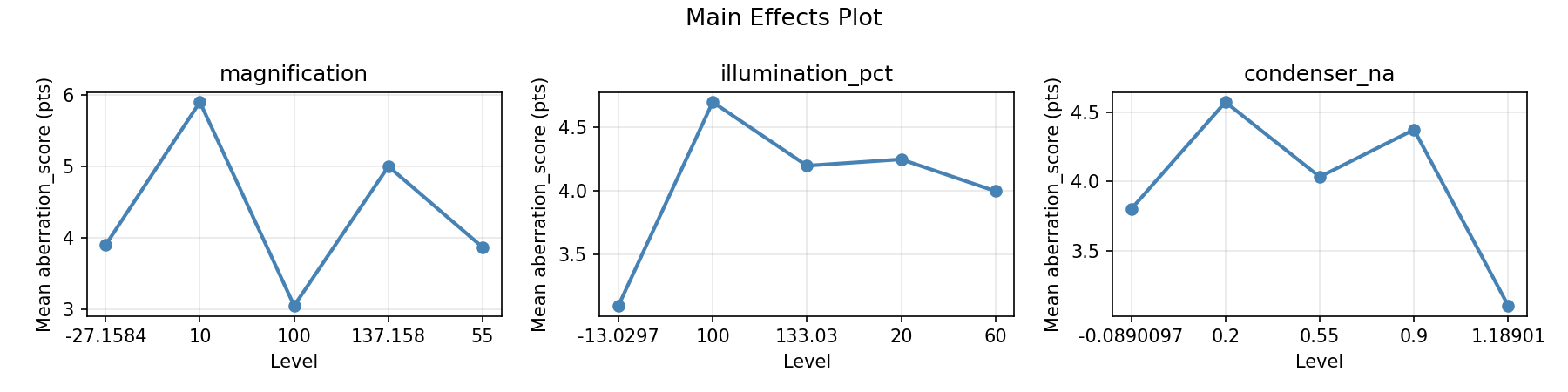
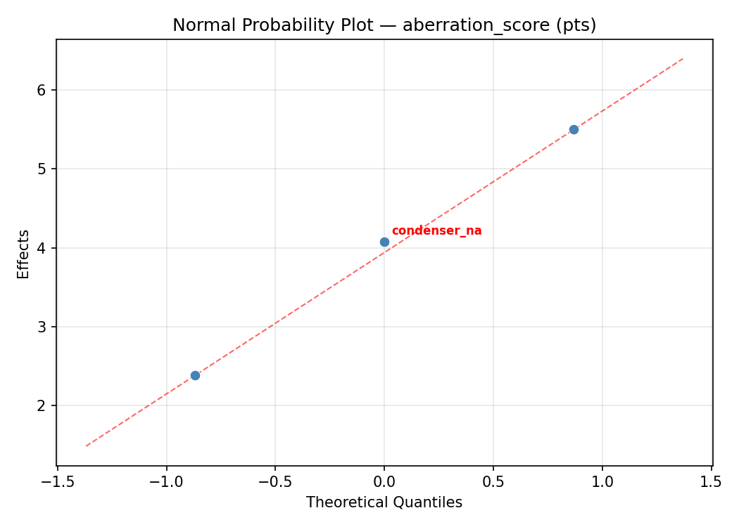
Response: aberration_score

Top factors: magnification (47.1%), illumination_pct (32.4%), condenser_na (20.6%).

ANOVA

Source	DF	SS	MS	F	p-value
Source	DF	SS	MS	F	p-value
magnification	4	12.5365	3.1341	1.409	0.3065
illumination_pct	4	6.7565	1.6891	0.759	0.5771
condenser_na	4	6.6857	1.6714	0.751	0.5816
Lack	of	Fit	2	3.9195	1.9597
Pure	Error	7	15.5750
Error	9	19.4945	2.2250
Total	21	45.4732	2.1654

Pareto Chart

Main Effects Plot

Normal Probability Plot of Effects

Normal probability plot for aberration_score

Half-Normal Plot of Effects

Model Diagnostics

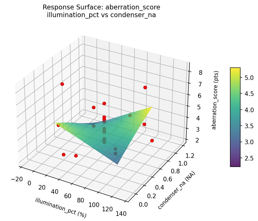
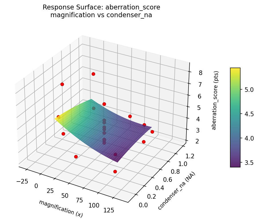
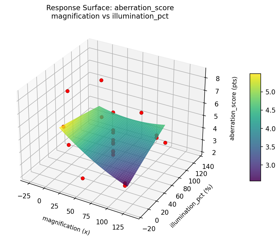
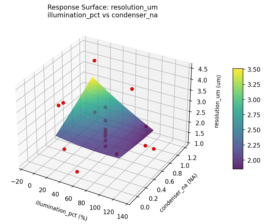
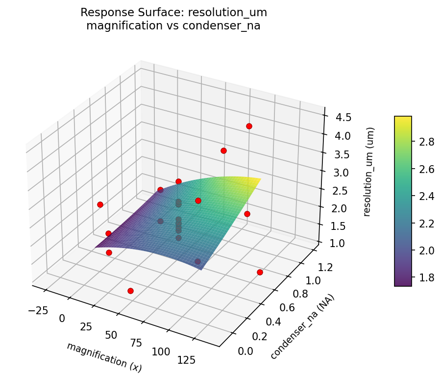
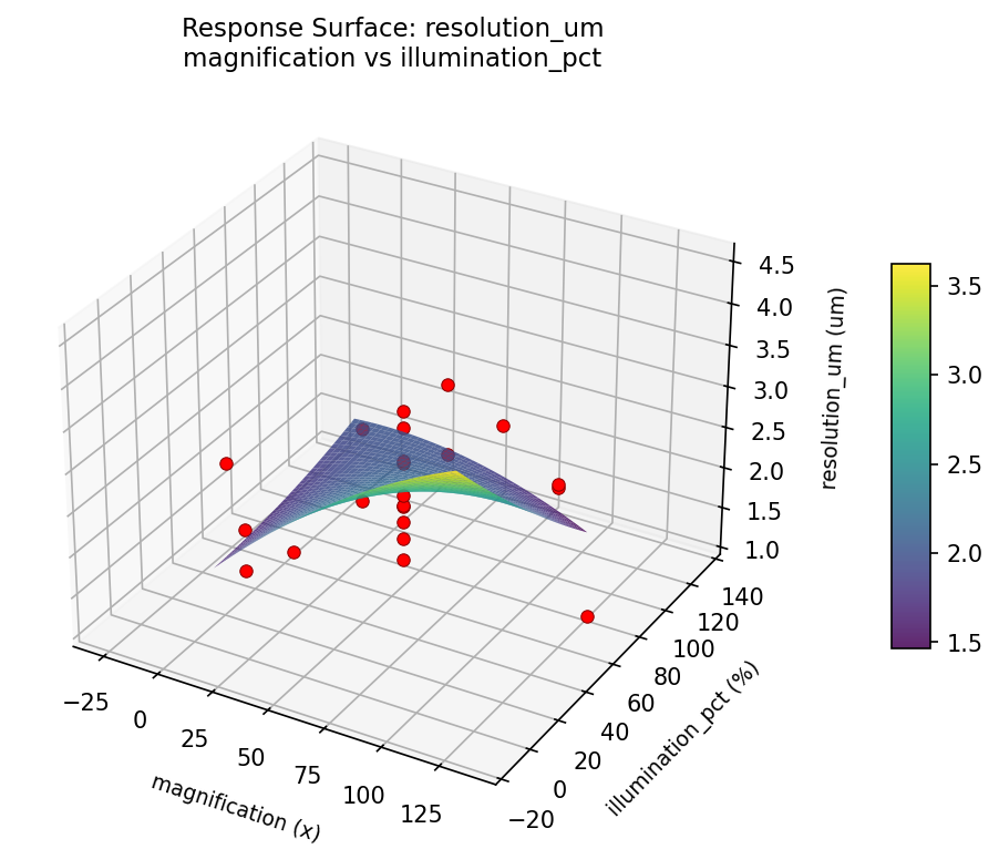
Response Surface Plots

3D surfaces fitted with quadratic RSM. Red dots are observed data points.

aberration score illumination pct vs condenser na

aberration score magnification vs condenser na

aberration score magnification vs illumination pct

resolution um illumination pct vs condenser na

resolution um magnification vs condenser na

resolution um magnification vs illumination pct

Multi-Objective Optimization

When responses compete, Derringer–Suich desirability finds the best compromise. Each response is scaled to a 0–1 desirability, then combined via a weighted geometric mean.

Overall Desirability

D = 0.7788

Per-Response Desirability

Response	Weight	Desirability	Predicted	Dir
`resolution_um`	1.0	0.8834	1.41 0.8834 1.41 um	↓
`aberration_score`	1.5	0.7161	3.80 0.7161 3.80 pts	↓

Recommended Settings

Factor	Value
`magnification`	55 x
`illumination_pct`	60 %
`condenser_na`	0.55 NA

Source: from observed run #17

Trade-off Summary

Sacrifice = how much worse than single-objective best.

Response	Predicted	Best Observed	Sacrifice
`aberration_score`	3.80	2.20	+1.60

Top 3 Runs by Desirability

Run	D	Factor Settings
#5	0.7229	magnification=100, illumination_pct=20, condenser_na=0.2
#22	0.7195	magnification=10, illumination_pct=20, condenser_na=0.9

Model Quality

Response	R²	Type
`aberration_score`	0.2484	linear

Full Multi-Objective Output

doe optimize --multi
============================================================
MULTI-OBJECTIVE OPTIMIZATION
Method: Derringer-Suich Desirability Function
============================================================

Overall desirability: D = 0.7788

Response                  Weight Desirability    Predicted  Direction
---------------------------------------------------------------------
resolution_um                1.0       0.8834        1.41 um   ↓
aberration_score             1.5       0.7161        3.80 pts   ↓

Recommended settings:
  magnification = 55 x
  illumination_pct = 60 %
  condenser_na = 0.55 NA
  (from observed run #17)

Trade-off summary:
  resolution_um: 1.41 (best observed: 1.15, sacrifice: +0.26)
  aberration_score: 3.80 (best observed: 2.20, sacrifice: +1.60)

Model quality:
  resolution_um: R² = 0.2431 (linear)
  aberration_score: R² = 0.2484 (linear)

Top 3 observed runs by overall desirability:
  1. Run #17 (D=0.7788): magnification=55, illumination_pct=60, condenser_na=0.55
  2. Run #5 (D=0.7229): magnification=100, illumination_pct=20, condenser_na=0.2
  3. Run #22 (D=0.7195): magnification=10, illumination_pct=20, condenser_na=0.9

Full Analysis Output

doe analyze
=== Main Effects: resolution_um ===
Factor                   Effect    Std Error   % Contribution
--------------------------------------------------------------
magnification            2.8025       0.1674            56.3%
illumination_pct         1.4525       0.1674            29.2%
condenser_na             0.7258       0.1674            14.6%

=== ANOVA Table: resolution_um ===
Source                      DF           SS           MS          F    p-value
-----------------------------------------------------------------------------
magnification                4       6.4469       1.6117      2.583     0.1092
illumination_pct             4       2.6316       0.6579      1.054     0.4322
condenser_na                 4       2.0290       0.5072      0.813     0.5477
Lack of Fit                  2       0.0000       0.0000      0.000     1.0000
Pure Error                   7       4.3685       0.6241
Error                        9       1.8325       0.6241
Total                       21      12.9399       0.6162

=== Summary Statistics: resolution_um ===

magnification:
  Level               N       Mean        Std        Min        Max
  ------------------------------------------------------------
  -27.1584            1     4.4700     0.0000     4.4700     4.4700
  10                  4     1.6675     0.2762     1.4100     2.0500
  100                 4     2.2075     0.2794     1.9600     2.6000
  137.158             1     1.9500     0.0000     1.9500     1.9500
  55                 12     2.3258     0.7404     1.1500     3.6700

illumination_pct:
  Level               N       Mean        Std        Min        Max
  ------------------------------------------------------------
  -13.0297            1     3.0200     0.0000     3.0200     3.0200
  100                 4     2.0975     0.4382     1.5400     2.6000
  133.03              1     3.2300     0.0000     3.2300     3.2300
  20                  4     1.7775     0.2975     1.4100     2.0700
  60                 12     2.3400     0.9277     1.1500     4.4700

condenser_na:
  Level               N       Mean        Std        Min        Max
  ------------------------------------------------------------
  -0.0890097          1     1.8800     0.0000     1.8800     1.8800
  0.2                 4     1.8050     0.3884     1.4100     2.2000
  0.55               12     2.5308     0.9537     1.1500     4.4700
  0.9                 4     2.0700     0.3888     1.6700     2.6000
  1.18901             1     2.0800     0.0000     2.0800     2.0800

=== Main Effects: aberration_score ===
Factor                   Effect    Std Error   % Contribution
--------------------------------------------------------------
magnification            3.2000       0.3137            47.1%
illumination_pct         2.2000       0.3137            32.4%
condenser_na             1.4000       0.3137            20.6%

=== ANOVA Table: aberration_score ===
Source                      DF           SS           MS          F    p-value
-----------------------------------------------------------------------------
magnification                4      12.5365       3.1341      1.409     0.3065
illumination_pct             4       6.7565       1.6891      0.759     0.5771
condenser_na                 4       6.6857       1.6714      0.751     0.5816
Lack of Fit                  2       3.9195       1.9597      0.881     0.4558
Pure Error                   7      15.5750       2.2250
Error                        9      19.4945       2.2250
Total                       21      45.4732       2.1654

=== Summary Statistics: aberration_score ===

magnification:
  Level               N       Mean        Std        Min        Max
  ------------------------------------------------------------
  -27.1584            1     2.4000     0.0000     2.4000     2.4000
  10                  4     5.6000     2.0928     3.8000     8.3000
  100                 4     3.8750     0.6898     3.0000     4.6000
  137.158             1     3.9000     0.0000     3.9000     3.9000
  55                 12     3.9083     1.2923     2.2000     7.1000

illumination_pct:
  Level               N       Mean        Std        Min        Max
  ------------------------------------------------------------
  -13.0297            1     3.1000     0.0000     3.1000     3.1000
  100                 4     5.0000     2.2993     3.0000     8.3000
  133.03              1     2.8000     0.0000     2.8000     2.8000
  20                  4     4.4750     1.1701     3.7000     6.2000
  60                 12     3.9417     1.3056     2.2000     7.1000

condenser_na:
  Level               N       Mean        Std        Min        Max
  ------------------------------------------------------------
  -0.0890097          1     4.8000     0.0000     4.8000     4.8000
  0.2                 4     5.1000     2.1710     3.7000     8.3000
  0.55               12     3.7000     1.3253     2.2000     7.1000
  0.9                 4     4.3750     1.3326     3.0000     6.2000
  1.18901             1     4.0000     0.0000     4.0000     4.0000

Optimization Recommendations

doe optimize
=== Optimization: resolution_um ===
Direction: minimize

Best observed run: #18
  magnification = 55
  illumination_pct = 60
  condenser_na = 0.55
  Value: 1.15

RSM Model (linear, R² = 0.0652, Adj R² = -0.0906):
  Coefficients:
    intercept                      +2.2650
    magnification                  -0.1182
    illumination_pct               -0.0570
    condenser_na                   -0.2008

RSM Model (quadratic, R² = 0.3994, Adj R² = -0.0511):
  Coefficients:
    intercept                      +1.9558
    magnification                  -0.1182
    illumination_pct               -0.0570
    condenser_na                   -0.2008
    magnification*illumination_pct +0.2350
    magnification*condenser_na     -0.3325
    illumination_pct*condenser_na  +0.0925
    magnification^2                -0.0724
    illumination_pct^2             +0.2711
    condenser_na^2                 +0.2651

  Curvature analysis:
    illumination_pct               coef=+0.2711  convex (has a minimum)
    condenser_na                   coef=+0.2651  convex (has a minimum)
    magnification                  coef=-0.0724  negligible curvature

  Notable interactions:
    magnification*condenser_na     coef=-0.3325  (antagonistic)

  Predicted optimum (from quadratic model, at observed points):
    magnification = 55
    illumination_pct = 60
    condenser_na = -0.0890097
    Predicted value: 3.2061

  Surface optimum (via L-BFGS-B, quadratic model):
    magnification = 100
    illumination_pct = 40.0439
    condenser_na = 0.9
    Predicted value: 1.4295

  Model quality: Weak fit — consider adding center points or using a different design.

Factor importance:
  1. condenser_na  (effect: 3.1, contribution: 57.5%)
  2. magnification  (effect: 1.1, contribution: 21.3%)
  3. illumination_pct  (effect: 1.1, contribution: 21.2%)

=== Optimization: aberration_score ===
Direction: minimize

Best observed run: #20
  magnification = 10
  illumination_pct = 20
  condenser_na = 0.9
  Value: 2.2

RSM Model (linear, R² = 0.0462, Adj R² = -0.1127):
  Coefficients:
    intercept                      +4.1409
    magnification                  -0.2830
    illumination_pct               +0.1195
    condenser_na                   +0.2214

RSM Model (quadratic, R² = 0.3714, Adj R² = -0.1001):
  Coefficients:
    intercept                      +4.6370
    magnification                  -0.2830
    illumination_pct               +0.1195
    condenser_na                   +0.2214
    magnification*illumination_pct -0.1125
    magnification*condenser_na     +0.2125
    illumination_pct*condenser_na  -0.0125
    magnification^2                +0.3170
    illumination_pct^2             -0.6430
    condenser_na^2                 -0.4180

  Curvature analysis:
    illumination_pct               coef=-0.6430  concave (has a maximum)
    condenser_na                   coef=-0.4180  concave (has a maximum)
    magnification                  coef=+0.3170  convex (has a minimum)

  Predicted optimum (from quadratic model, at observed points):
    magnification = -27.1584
    illumination_pct = 60
    condenser_na = 0.55
    Predicted value: 6.2102

  Surface optimum (via L-BFGS-B, quadratic model):
    magnification = 82.1866
    illumination_pct = 20
    condenser_na = 0.2
    Predicted value: 3.1069

  Model quality: Weak fit — consider adding center points or using a different design.

Factor importance:
  1. magnification  (effect: 5.3, contribution: 53.5%)
  2. condenser_na  (effect: 2.6, contribution: 26.5%)
  3. illumination_pct  (effect: 2.0, contribution: 20.0%)