Titration Accuracy Optimization

Summary

This experiment investigates titration accuracy optimization. Box-Behnken design to maximize endpoint precision and minimize reagent waste by tuning drop size, stirring speed, and indicator concentration.

The design varies 3 factors: drop size ul (uL), ranging from 10 to 100, stir rpm (rpm), ranging from 100 to 600, and indicator pct (%), ranging from 0.05 to 0.5. The goal is to optimize 2 responses: precision pct (%) (maximize) and reagent waste ml (mL) (minimize). Fixed conditions held constant across all runs include analyte = HCl, titrant = NaOH.

A Box-Behnken design was chosen because it efficiently fits quadratic models with 3 continuous factors while avoiding extreme corner combinations — requiring only 15 runs instead of the 8 needed for a full factorial at two levels.

Quadratic response surface models were fitted to capture potential curvature and factor interactions. The RSM contour plots below visualize how pairs of factors jointly affect each response.

Key Findings

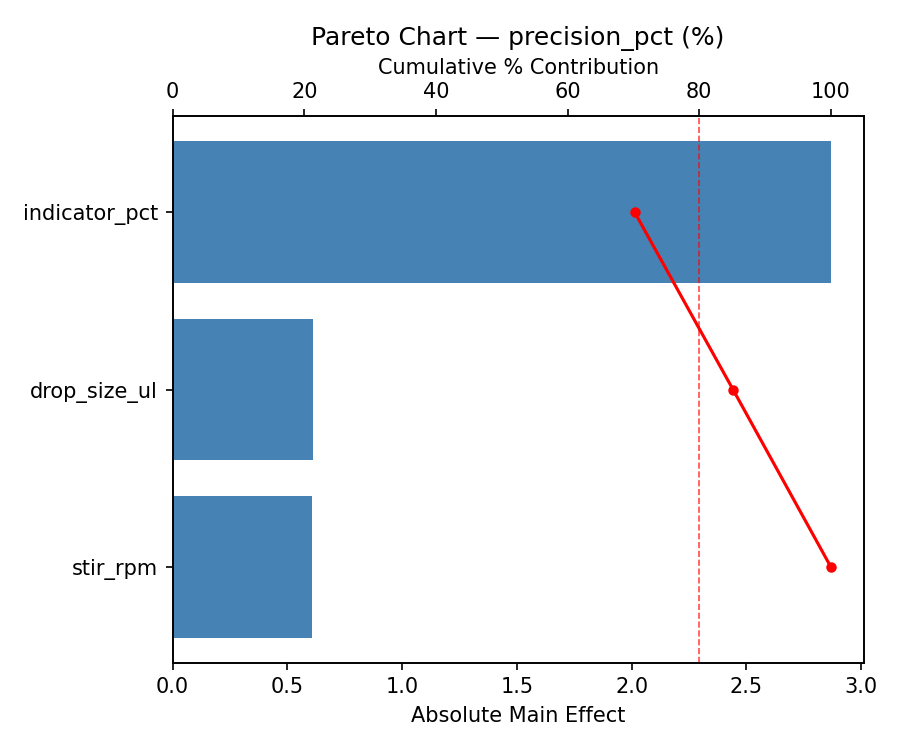
For precision pct, the most influential factors were drop size ul (44.3%), indicator pct (34.1%), stir rpm (21.6%). The best observed value was 99.3 (at drop size ul = 55, stir rpm = 100, indicator pct = 0.05).

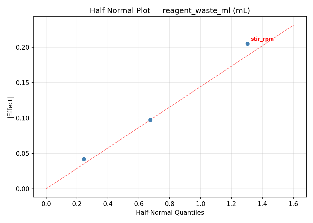
For reagent waste ml, the most influential factors were drop size ul (55.3%), stir rpm (25.1%), indicator pct (19.6%). The best observed value was 0.21 (at drop size ul = 55, stir rpm = 600, indicator pct = 0.05).

Recommended Next Steps

Run confirmation experiments at the predicted optimal settings to validate the model.
Consider whether any fixed factors should be varied in a future study.

Experimental Setup

Factors

Factor	Low	High	Unit
`drop_size_ul`	10	100	uL
`stir_rpm`	100	600	rpm
`indicator_pct`	0.05	0.5	%

Fixed: analyte = HCl, titrant = NaOH

Responses

Response	Direction	Unit
`precision_pct`	↑ maximize	%
`reagent_waste_ml`	↓ minimize	mL

Configuration

use_cases/187_titration_accuracy/config.json

{
  "metadata": {
    "name": "Titration Accuracy Optimization",
    "description": "Box-Behnken design to maximize endpoint precision and minimize reagent waste by tuning drop size, stirring speed, and indicator concentration"
  },
  "factors": [
    {
      "name": "drop_size_ul",
      "levels": [
        "10",
        "100"
      ],
      "type": "continuous",
      "unit": "uL"
    },
    {
      "name": "stir_rpm",
      "levels": [
        "100",
        "600"
      ],
      "type": "continuous",
      "unit": "rpm"
    },
    {
      "name": "indicator_pct",
      "levels": [
        "0.05",
        "0.5"
      ],
      "type": "continuous",
      "unit": "%"
    }
  ],
  "fixed_factors": {
    "analyte": "HCl",
    "titrant": "NaOH"
  },
  "responses": [
    {
      "name": "precision_pct",
      "optimize": "maximize",
      "unit": "%"
    },
    {
      "name": "reagent_waste_ml",
      "optimize": "minimize",
      "unit": "mL"
    }
  ],
  "settings": {
    "operation": "box_behnken",
    "test_script": "use_cases/187_titration_accuracy/sim.sh"
  }
}

Experimental Matrix

The Box-Behnken Design produces 15 runs. Each row is one experiment with specific factor settings.

Run	`drop_size_ul`	`stir_rpm`	`indicator_pct`
1	55	100	0.05
2	55	350	0.275
3	100	350	0.5
4	100	350	0.05
5	55	350	0.275
6	55	350	0.275
7	10	350	0.5
8	100	100	0.275
9	55	100	0.5
10	100	600	0.275
11	10	350	0.05
12	55	600	0.5
13	10	100	0.275
14	10	600	0.275
15	55	600	0.05

Step-by-Step Workflow

1

Preview the design

Terminal

$ doe info --config use_cases/187_titration_accuracy/config.json

2

Generate the runner script

Terminal

$ doe generate --config use_cases/187_titration_accuracy/config.json \
    --output use_cases/187_titration_accuracy/results/run.sh --seed 42

3

Execute the experiments

Terminal

$ bash use_cases/187_titration_accuracy/results/run.sh

4

Analyze results

Terminal

$ doe analyze --config use_cases/187_titration_accuracy/config.json

5

Get optimization recommendations

Terminal

$ doe optimize --config use_cases/187_titration_accuracy/config.json

6

Multi-objective optimization

With 2 competing responses, use --multi to find the best compromise via Derringer–Suich desirability.

Terminal

$ doe optimize --config use_cases/187_titration_accuracy/config.json --multi

7

Generate the HTML report

Terminal

$ doe report --config use_cases/187_titration_accuracy/config.json \
    --output use_cases/187_titration_accuracy/results/report.html

Features Exercised

Feature	Value
Design type	`box_behnken`
Factor types	`continuous` (all 3)
Arg style	`double-dash`
Responses	2 (precision_pct ↑, reagent_waste_ml ↓)
Total runs	15

Analysis Results

Generated from actual experiment runs using the DOE Helper Tool.

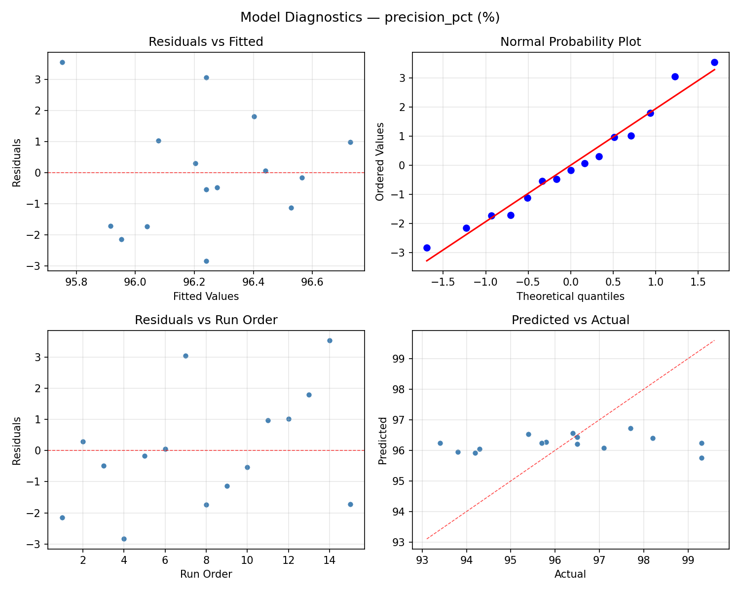
Response: precision_pct

Top factors: drop_size_ul (44.3%), indicator_pct (34.1%), stir_rpm (21.6%).

ANOVA

Source	DF	SS	MS	F	p-value
Source	DF	SS	MS	F	p-value
drop_size_ul	2	7.4317	3.7159	0.570	0.5870
stir_rpm	2	2.2267	1.1134	0.171	0.8460
indicator_pct	2	5.2410	2.6205	0.402	0.6818
Lack	of	Fit	6	20.7966	3.4661
Pure	Error	2	13.0400
Error	8	33.8366	6.5200
Total	14	48.7360	3.4811

Pareto Chart

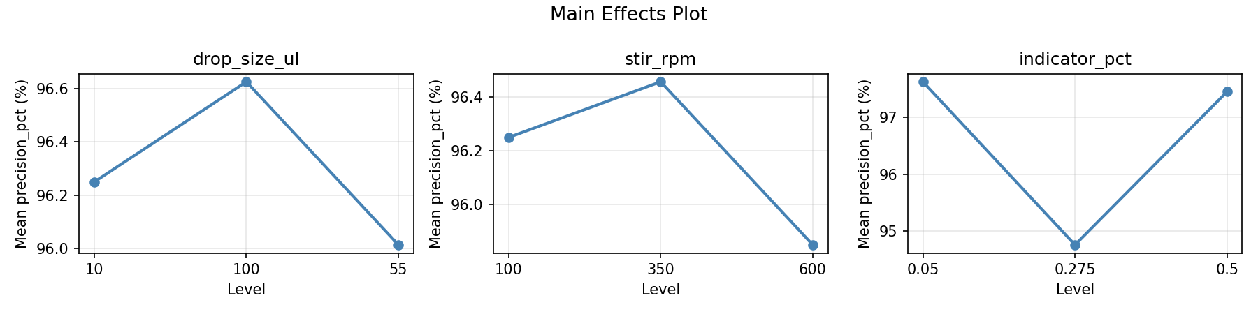
Main Effects Plot

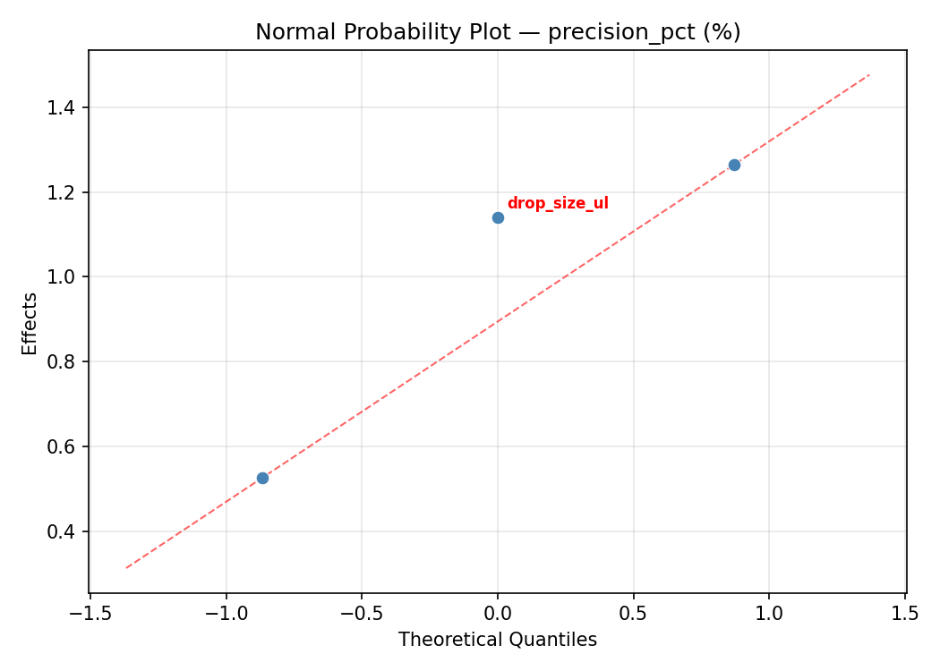
Normal Probability Plot of Effects

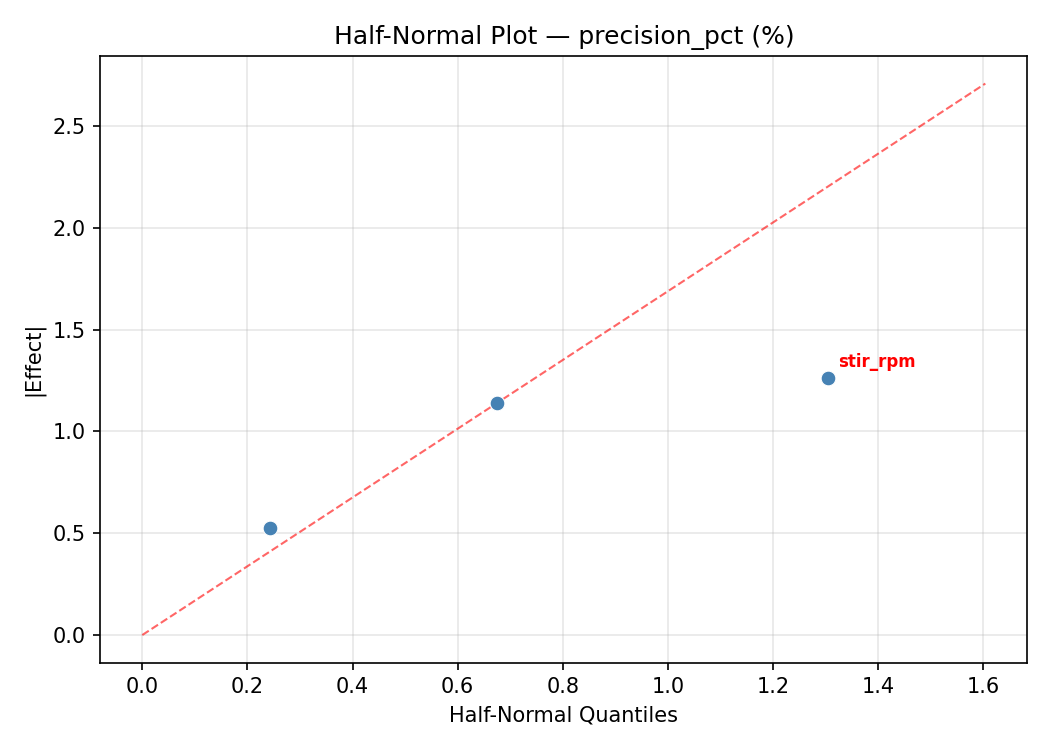
Normal probability plot for precision_pct

Half-Normal Plot of Effects

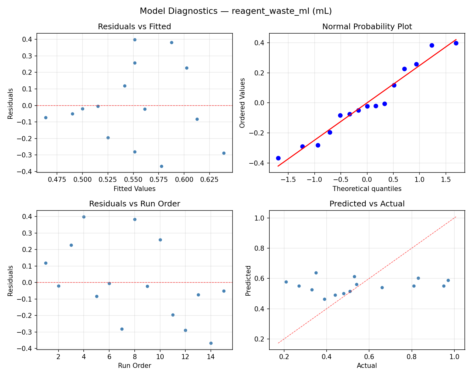
Model Diagnostics

Response: reagent_waste_ml

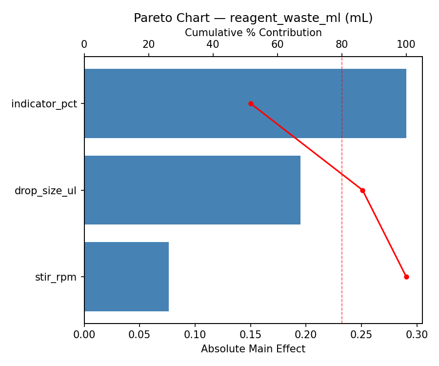
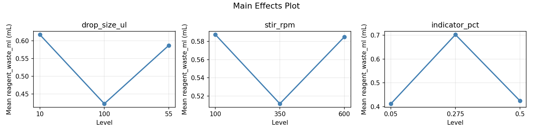
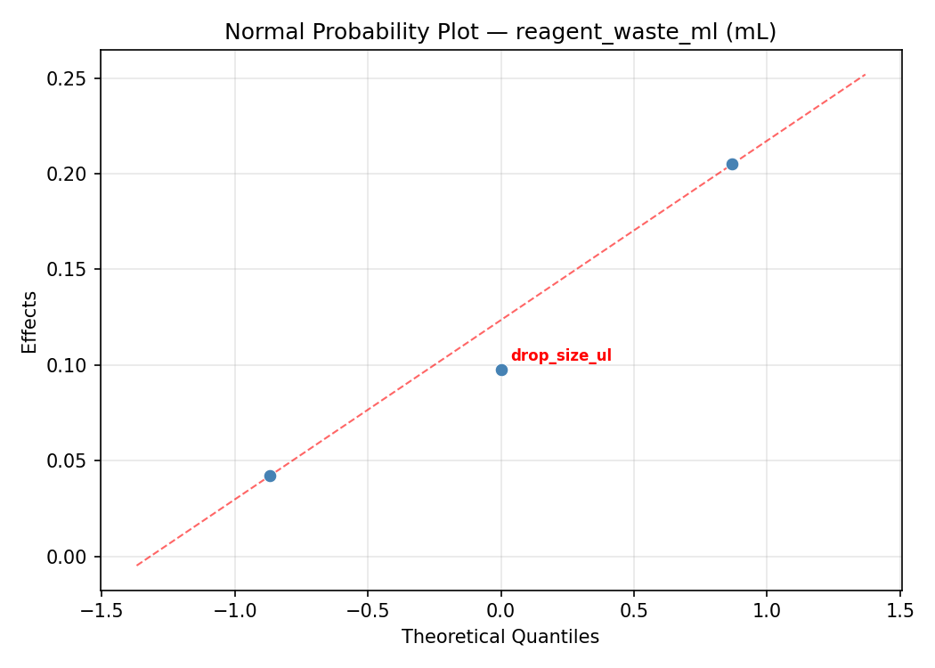
Top factors: drop_size_ul (55.3%), stir_rpm (25.1%), indicator_pct (19.6%).

ANOVA

Source	DF	SS	MS	F	p-value
Source	DF	SS	MS	F	p-value
drop_size_ul	2	0.2166	0.1083	0.720	0.5160
stir_rpm	2	0.0617	0.0309	0.205	0.8188
indicator_pct	2	0.0339	0.0169	0.113	0.8950
Lack	of	Fit	6	0.2083	0.0347
Pure	Error	2	0.3011
Error	8	0.5094	0.1505
Total	14	0.8216	0.0587

Pareto Chart

Main Effects Plot

Normal Probability Plot of Effects

Normal probability plot for reagent_waste_ml

Half-Normal Plot of Effects

Model Diagnostics

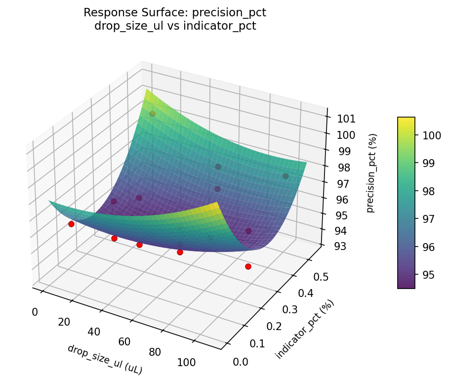
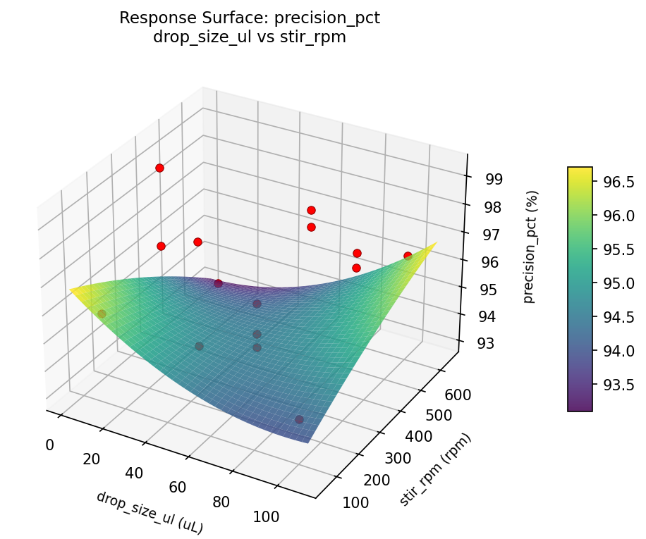
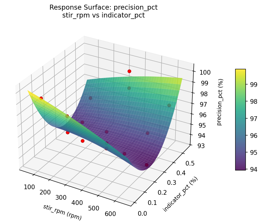
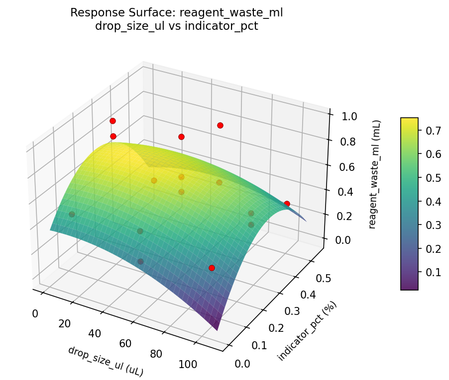
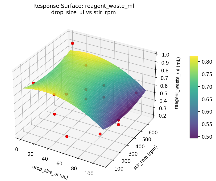
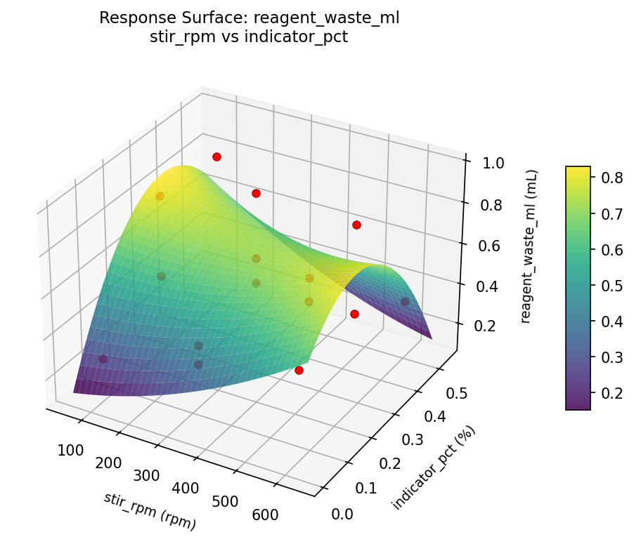
Response Surface Plots

3D surfaces fitted with quadratic RSM. Red dots are observed data points.

precision pct drop size ul vs indicator pct

precision pct drop size ul vs stir rpm

precision pct stir rpm vs indicator pct

reagent waste ml drop size ul vs indicator pct

reagent waste ml drop size ul vs stir rpm

reagent waste ml stir rpm vs indicator pct

Multi-Objective Optimization

When responses compete, Derringer–Suich desirability finds the best compromise. Each response is scaled to a 0–1 desirability, then combined via a weighted geometric mean.

Overall Desirability

D = 0.9545

Per-Response Desirability

Response	Weight	Desirability	Predicted	Dir
`precision_pct`	1.5	0.9545	99.30 0.9545 99.30 %	↑
`reagent_waste_ml`	1.0	0.9545	0.21 0.9545 0.21 mL	↓

Recommended Settings

Factor	Value
`drop_size_ul`	55 uL
`stir_rpm`	100 rpm
`indicator_pct`	0.05 %

Source: from observed run #14

Trade-off Summary

Sacrifice = how much worse than single-objective best.

Response	Predicted	Best Observed	Sacrifice
`reagent_waste_ml`	0.21	0.21	+0.00

Top 3 Runs by Desirability

Run	D	Factor Settings
#7	0.9252	drop_size_ul=100, stir_rpm=350, indicator_pct=0.5
#13	0.7664	drop_size_ul=55, stir_rpm=350, indicator_pct=0.275

Model Quality

Response	R²	Type
`reagent_waste_ml`	0.7534	quadratic

Full Multi-Objective Output

doe optimize --multi
============================================================
MULTI-OBJECTIVE OPTIMIZATION
Method: Derringer-Suich Desirability Function
============================================================

Overall desirability: D = 0.9545

Response                  Weight Desirability    Predicted  Direction
---------------------------------------------------------------------
precision_pct                1.5       0.9545       99.30 %   ↑
reagent_waste_ml             1.0       0.9545        0.21 mL   ↓

Recommended settings:
  drop_size_ul = 55 uL
  stir_rpm = 100 rpm
  indicator_pct = 0.05 %
  (from observed run #14)

Trade-off summary:
  precision_pct: 99.30 (best observed: 99.30, sacrifice: +0.00)
  reagent_waste_ml: 0.21 (best observed: 0.21, sacrifice: +0.00)

Model quality:
  precision_pct: R² = 0.6602 (quadratic)
  reagent_waste_ml: R² = 0.7534 (quadratic)

Top 3 observed runs by overall desirability:
  1. Run #14 (D=0.9545): drop_size_ul=55, stir_rpm=100, indicator_pct=0.05
  2. Run #7 (D=0.9252): drop_size_ul=100, stir_rpm=350, indicator_pct=0.5
  3. Run #13 (D=0.7664): drop_size_ul=55, stir_rpm=350, indicator_pct=0.275

Full Analysis Output

doe analyze
=== Main Effects: precision_pct ===
Factor                   Effect    Std Error   % Contribution
--------------------------------------------------------------
drop_size_ul             1.8500       0.4817            44.3%
indicator_pct            1.4250       0.4817            34.1%
stir_rpm                 0.9036       0.4817            21.6%

=== ANOVA Table: precision_pct ===
Source                      DF           SS           MS          F    p-value
-----------------------------------------------------------------------------
drop_size_ul                 2       7.4317       3.7159      0.570     0.5870
stir_rpm                     2       2.2267       1.1134      0.171     0.8460
indicator_pct                2       5.2410       2.6205      0.402     0.6818
Lack of Fit                  6      20.7966       3.4661      0.532     0.7678
Pure Error                   2      13.0400       6.5200
Error                        8      33.8366       6.5200
Total                       14      48.7360       3.4811

=== Summary Statistics: precision_pct ===

drop_size_ul:
  Level               N       Mean        Std        Min        Max
  ------------------------------------------------------------
  10                  4    95.5000     1.5384    93.4000    97.1000
  100                 4    97.3500     1.7369    95.4000    99.3000
  55                  7    96.0286     2.0475    93.8000    99.3000

stir_rpm:
  Level               N       Mean        Std        Min        Max
  ------------------------------------------------------------
  100                 4    96.0750     1.2816    94.2000    97.1000
  350                 7    96.6286     1.7905    94.3000    99.3000
  600                 4    95.7250     2.7293    93.4000    99.3000

indicator_pct:
  Level               N       Mean        Std        Min        Max
  ------------------------------------------------------------
  0.05                4    95.3750     1.1442    93.8000    96.5000
  0.275               7    96.8000     2.2840    93.4000    99.3000
  0.5                 4    96.1250     1.6601    94.2000    98.2000

=== Main Effects: reagent_waste_ml ===
Factor                   Effect    Std Error   % Contribution
--------------------------------------------------------------
drop_size_ul             0.3225       0.0625            55.3%
stir_rpm                 0.1464       0.0625            25.1%
indicator_pct            0.1146       0.0625            19.6%

=== ANOVA Table: reagent_waste_ml ===
Source                      DF           SS           MS          F    p-value
-----------------------------------------------------------------------------
drop_size_ul                 2       0.2166       0.1083      0.720     0.5160
stir_rpm                     2       0.0617       0.0309      0.205     0.8188
indicator_pct                2       0.0339       0.0169      0.113     0.8950
Lack of Fit                  6       0.2083       0.0347      0.231     0.9316
Pure Error                   2       0.3011       0.1505
Error                        8       0.5094       0.1505
Total                       14       0.8216       0.0587

=== Summary Statistics: reagent_waste_ml ===

drop_size_ul:
  Level               N       Mean        Std        Min        Max
  ------------------------------------------------------------
  10                  4     0.7350     0.2640     0.3500     0.9500
  100                 4     0.4125     0.1497     0.2100     0.5400
  55                  7     0.5257     0.2340     0.2700     0.9700

stir_rpm:
  Level               N       Mean        Std        Min        Max
  ------------------------------------------------------------
  100                 4     0.4450     0.0695     0.3500     0.5100
  350                 7     0.5914     0.2778     0.2700     0.9700
  600                 4     0.5875     0.3069     0.2100     0.9500

indicator_pct:
  Level               N       Mean        Std        Min        Max
  ------------------------------------------------------------
  0.05                4     0.6275     0.1544     0.4800     0.8300
  0.275               7     0.5129     0.3190     0.2100     0.9700
  0.5                 4     0.5425     0.1875     0.3900     0.8100

Optimization Recommendations

doe optimize
=== Optimization: precision_pct ===
Direction: maximize

Best observed run: #7
  drop_size_ul = 55
  stir_rpm = 100
  indicator_pct = 0.05
  Value: 99.3

RSM Model (linear, R² = 0.3736, Adj R² = 0.2028):
  Coefficients:
    intercept                      +96.2400
    drop_size_ul                   -0.4750
    stir_rpm                       -0.4000
    indicator_pct                  -1.3750

RSM Model (quadratic, R² = 0.6673, Adj R² = 0.0683):
  Coefficients:
    intercept                      +95.9333
    drop_size_ul                   -0.4750
    stir_rpm                       -0.4000
    indicator_pct                  -1.3750
    drop_size_ul*stir_rpm          +0.0500
    drop_size_ul*indicator_pct     +0.9000
    stir_rpm*indicator_pct         -0.5000
    drop_size_ul^2                 -0.3417
    stir_rpm^2                     -0.5417
    indicator_pct^2                +1.4583

  Curvature analysis:
    indicator_pct                  coef=+1.4583  convex (has a minimum)
    stir_rpm                       coef=-0.5417  concave (has a maximum)
    drop_size_ul                   coef=-0.3417  concave (has a maximum)

  Notable interactions:
    drop_size_ul*indicator_pct     coef=+0.9000  (synergistic)
    stir_rpm*indicator_pct         coef=-0.5000  (antagonistic)

  Predicted optimum (from linear model, at observed points):
    drop_size_ul = 10
    stir_rpm = 350
    indicator_pct = 0.05
    Predicted value: 98.0900

  Surface optimum (via L-BFGS-B, linear model):
    drop_size_ul = 10
    stir_rpm = 100
    indicator_pct = 0.05
    Predicted value: 98.4900

  Model quality: Weak fit — consider adding center points or using a different design.

Factor importance:
  1. indicator_pct  (effect: 2.9, contribution: 59.5%)
  2. stir_rpm  (effect: 1.0, contribution: 21.0%)
  3. drop_size_ul  (effect: 1.0, contribution: 19.5%)

=== Optimization: reagent_waste_ml ===
Direction: minimize

Best observed run: #14
  drop_size_ul = 55
  stir_rpm = 600
  indicator_pct = 0.05
  Value: 0.21

RSM Model (linear, R² = 0.2622, Adj R² = 0.0610):
  Coefficients:
    intercept                      +0.5513
    drop_size_ul                   -0.0113
    stir_rpm                       +0.0400
    indicator_pct                  +0.1588

RSM Model (quadratic, R² = 0.8134, Adj R² = 0.4774):
  Coefficients:
    intercept                      +0.4233
    drop_size_ul                   -0.0112
    stir_rpm                       +0.0400
    indicator_pct                  +0.1587
    drop_size_ul*stir_rpm          -0.1475
    drop_size_ul*indicator_pct     -0.1550
    stir_rpm*indicator_pct         +0.1175
    drop_size_ul^2                 +0.1708
    stir_rpm^2                     +0.1483
    indicator_pct^2                -0.0792

  Curvature analysis:
    drop_size_ul                   coef=+0.1708  convex (has a minimum)
    stir_rpm                       coef=+0.1483  convex (has a minimum)
    indicator_pct                  coef=-0.0792  negligible curvature

  Predicted optimum (from quadratic model, at observed points):
    drop_size_ul = 10
    stir_rpm = 600
    indicator_pct = 0.275
    Predicted value: 0.9412

  Surface optimum (via L-BFGS-B, quadratic model):
    drop_size_ul = 37.3546
    stir_rpm = 366.569
    indicator_pct = 0.05
    Predicted value: 0.1547

  Model quality: Good fit — general trends are captured, some noise remains.

Factor importance:
  1. indicator_pct  (effect: 0.3, contribution: 46.9%)
  2. stir_rpm  (effect: 0.2, contribution: 26.9%)
  3. drop_size_ul  (effect: 0.2, contribution: 26.2%)