Summary
This experiment investigates moving day logistics. Box-Behnken design to minimize total move time and breakage by tuning box size, crew size, and truck loading strategy padding thickness.
The design varies 3 factors: box volume L (L), ranging from 30 to 80, crew size (people), ranging from 2 to 6, and padding layers (layers), ranging from 1 to 4. The goal is to optimize 2 responses: total hours (hrs) (minimize) and breakage pct (%) (minimize). Fixed conditions held constant across all runs include distance km = 20, apartment floor = 3.
A Box-Behnken design was chosen because it efficiently fits quadratic models with 3 continuous factors while avoiding extreme corner combinations — requiring only 15 runs instead of the 8 needed for a full factorial at two levels.
Quadratic response surface models were fitted to capture potential curvature and factor interactions. The RSM contour plots below visualize how pairs of factors jointly affect each response.
Key Findings
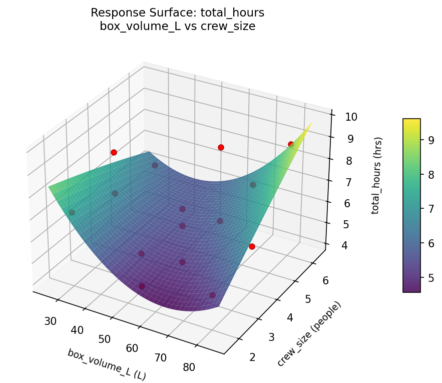
For total hours, the most influential factors were box volume L (61.0%), crew size (33.8%), padding layers (5.1%). The best observed value was 4.1 (at box volume L = 80, crew size = 4, padding layers = 4).
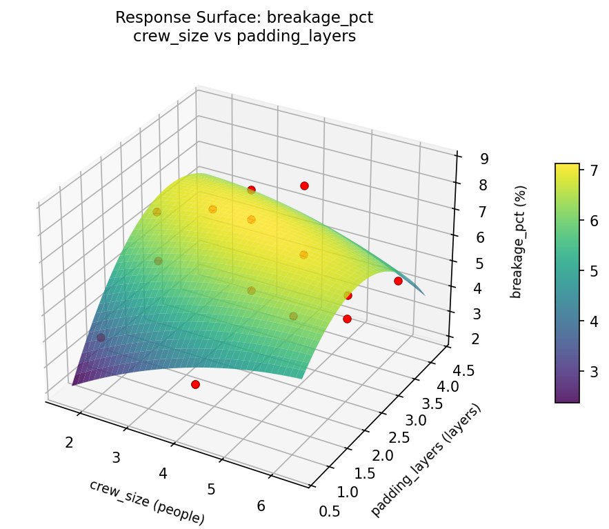
For breakage pct, the most influential factors were padding layers (43.5%), box volume L (29.8%), crew size (26.6%). The best observed value was 3.2 (at box volume L = 55, crew size = 4, padding layers = 2.5).
Recommended Next Steps
- Run confirmation experiments at the predicted optimal settings to validate the model.
- Consider whether any fixed factors should be varied in a future study.
Experimental Setup
Factors
| Factor | Low | High | Unit |
|---|
box_volume_L | 30 | 80 | L |
crew_size | 2 | 6 | people |
padding_layers | 1 | 4 | layers |
Fixed: distance_km = 20, apartment_floor = 3
Responses
| Response | Direction | Unit |
|---|
total_hours | ↓ minimize | hrs |
breakage_pct | ↓ minimize | % |
Configuration
{
"metadata": {
"name": "Moving Day Logistics",
"description": "Box-Behnken design to minimize total move time and breakage by tuning box size, crew size, and truck loading strategy padding thickness"
},
"factors": [
{
"name": "box_volume_L",
"levels": [
"30",
"80"
],
"type": "continuous",
"unit": "L"
},
{
"name": "crew_size",
"levels": [
"2",
"6"
],
"type": "continuous",
"unit": "people"
},
{
"name": "padding_layers",
"levels": [
"1",
"4"
],
"type": "continuous",
"unit": "layers"
}
],
"fixed_factors": {
"distance_km": "20",
"apartment_floor": "3"
},
"responses": [
{
"name": "total_hours",
"optimize": "minimize",
"unit": "hrs"
},
{
"name": "breakage_pct",
"optimize": "minimize",
"unit": "%"
}
],
"settings": {
"operation": "box_behnken",
"test_script": "use_cases/197_moving_day_logistics/sim.sh"
}
}
Experimental Matrix
The Box-Behnken Design produces 15 runs. Each row is one experiment with specific factor settings.
| Run | box_volume_L | crew_size | padding_layers |
|---|
| 1 | 55 | 2 | 1 |
| 2 | 55 | 4 | 2.5 |
| 3 | 80 | 4 | 4 |
| 4 | 80 | 4 | 1 |
| 5 | 55 | 4 | 2.5 |
| 6 | 55 | 4 | 2.5 |
| 7 | 30 | 4 | 4 |
| 8 | 80 | 2 | 2.5 |
| 9 | 55 | 2 | 4 |
| 10 | 80 | 6 | 2.5 |
| 11 | 30 | 4 | 1 |
| 12 | 55 | 6 | 4 |
| 13 | 30 | 2 | 2.5 |
| 14 | 30 | 6 | 2.5 |
| 15 | 55 | 6 | 1 |
Step-by-Step Workflow
1
Preview the design
$ doe info --config use_cases/197_moving_day_logistics/config.json
2
Generate the runner script
$ doe generate --config use_cases/197_moving_day_logistics/config.json \
--output use_cases/197_moving_day_logistics/results/run.sh --seed 42
3
Execute the experiments
$ bash use_cases/197_moving_day_logistics/results/run.sh
4
Analyze results
$ doe analyze --config use_cases/197_moving_day_logistics/config.json
5
Get optimization recommendations
$ doe optimize --config use_cases/197_moving_day_logistics/config.json
6
Multi-objective optimization
With 2 competing responses, use --multi to find the best compromise via Derringer–Suich desirability.
$ doe optimize --config use_cases/197_moving_day_logistics/config.json --multi
7
Generate the HTML report
$ doe report --config use_cases/197_moving_day_logistics/config.json \
--output use_cases/197_moving_day_logistics/results/report.html
Features Exercised
| Feature | Value |
|---|
| Design type | box_behnken |
| Factor types | continuous (all 3) |
| Arg style | double-dash |
| Responses | 2 (total_hours ↓, breakage_pct ↓) |
| Total runs | 15 |
Analysis Results
Generated from actual experiment runs using the DOE Helper Tool.
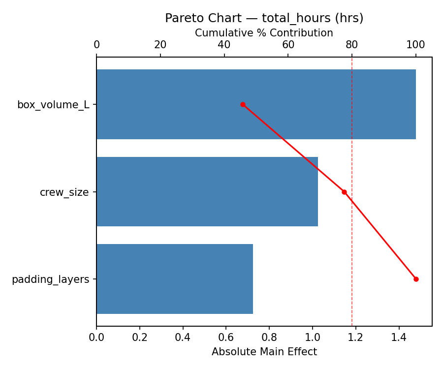
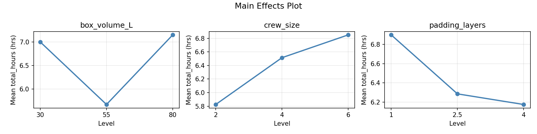
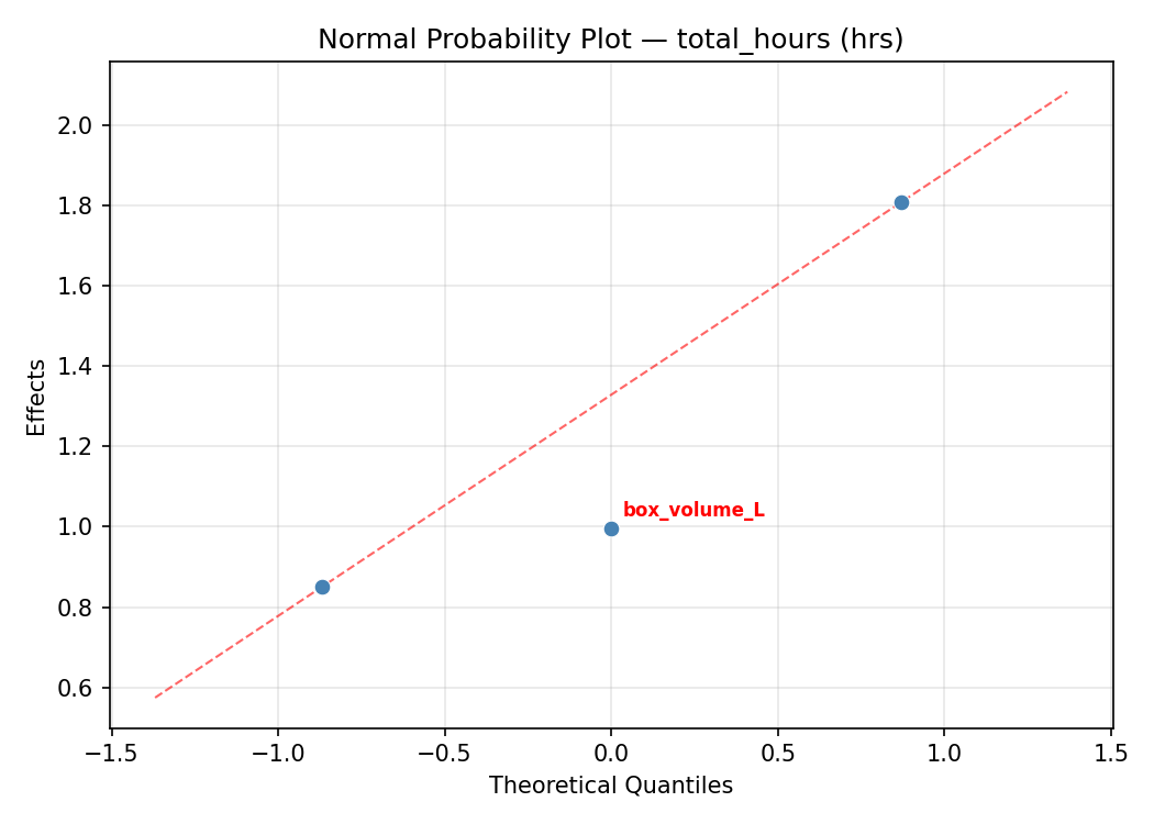
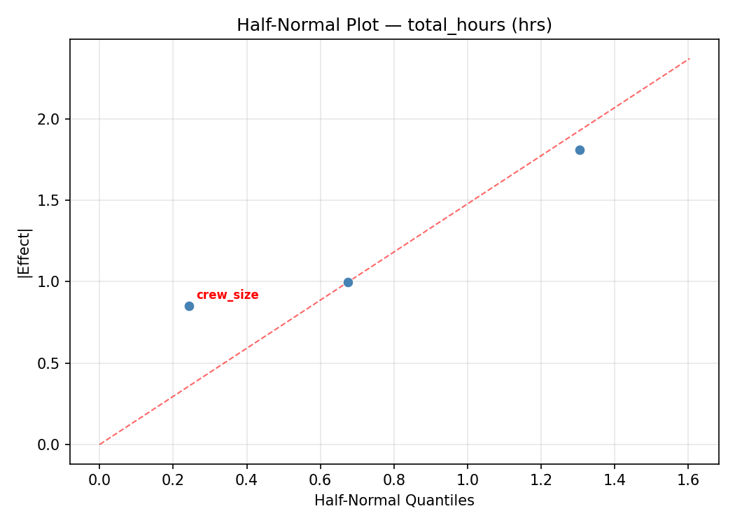
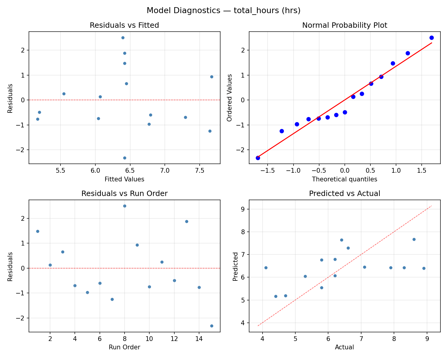
Response: total_hours
Top factors: box_volume_L (61.0%), crew_size (33.8%), padding_layers (5.1%).
ANOVA
| Source | DF | SS | MS | F | p-value |
|---|
| Source | DF | SS | MS | F | p-value |
| box_volume_L | 2 | 9.2465 | 4.6233 | 3.035 | 0.1045 |
| crew_size | 2 | 2.7547 | 1.3774 | 0.904 | 0.4426 |
| padding_layers | 2 | 0.0622 | 0.0311 | 0.020 | 0.9798 |
| Lack | of | Fit | 6 | 16.5539 | 2.7590 |
| Pure | Error | 2 | 3.0467 | | |
| Error | 8 | 19.6006 | 1.5233 | | |
| Total | 14 | 31.6640 | 2.2617 | | |
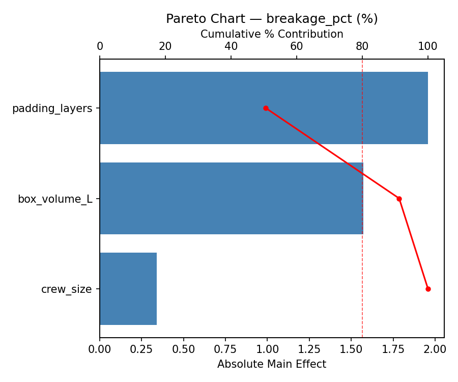
Pareto Chart
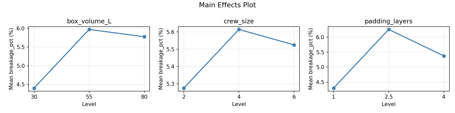
Main Effects Plot
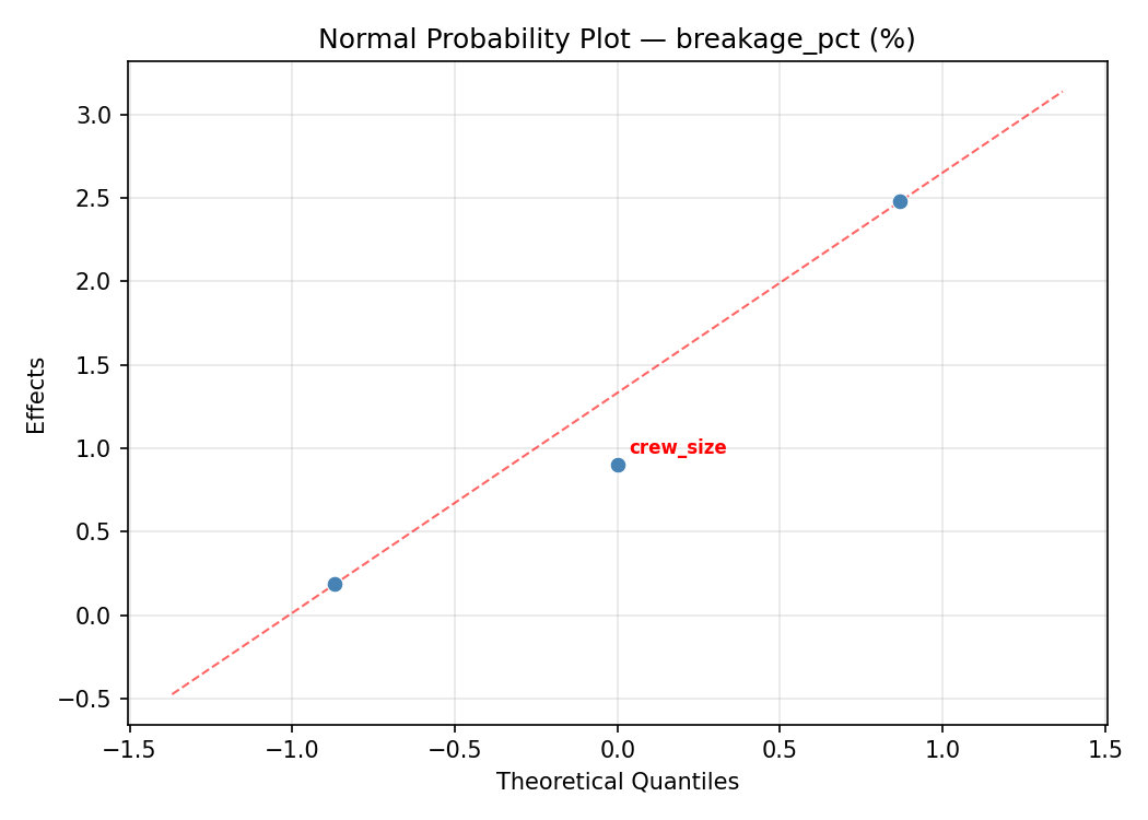
Normal Probability Plot of Effects
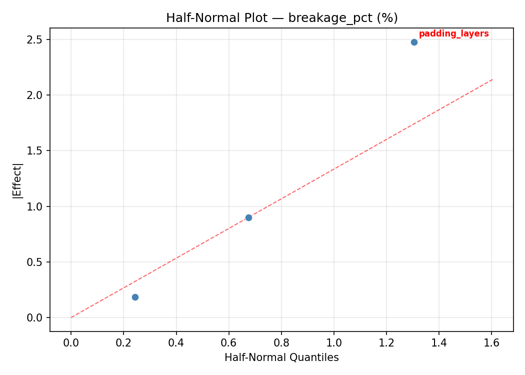
Half-Normal Plot of Effects
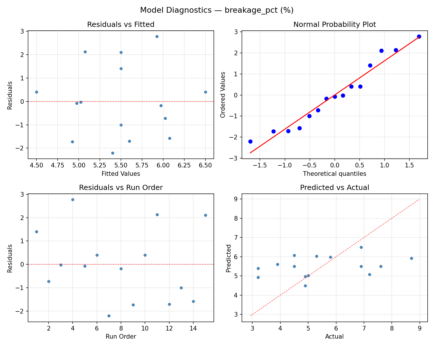
Model Diagnostics
Response: breakage_pct
Top factors: padding_layers (43.5%), box_volume_L (29.8%), crew_size (26.6%).
ANOVA
| Source | DF | SS | MS | F | p-value |
|---|
| Source | DF | SS | MS | F | p-value |
| box_volume_L | 2 | 3.8482 | 1.9241 | 2.337 | 0.1587 |
| crew_size | 2 | 5.2057 | 2.6029 | 3.161 | 0.0973 |
| padding_layers | 2 | 11.4854 | 5.7427 | 6.975 | 0.0176 |
| Lack | of | Fit | 6 | 15.5140 | 2.5857 |
| Pure | Error | 2 | 1.6467 | | |
| Error | 8 | 17.1607 | 0.8233 | | |
| Total | 14 | 37.7000 | 2.6929 | | |
Pareto Chart
Main Effects Plot
Normal Probability Plot of Effects
Half-Normal Plot of Effects
Model Diagnostics
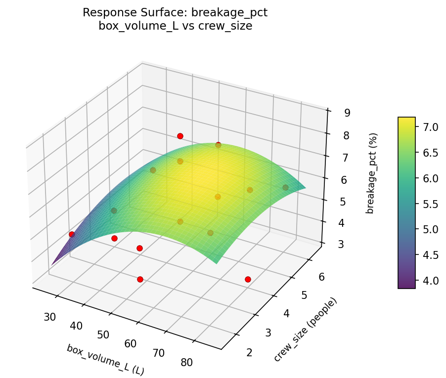
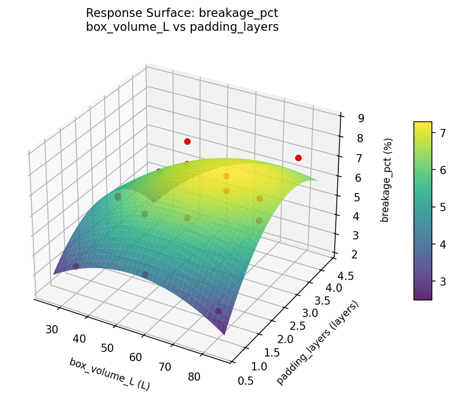
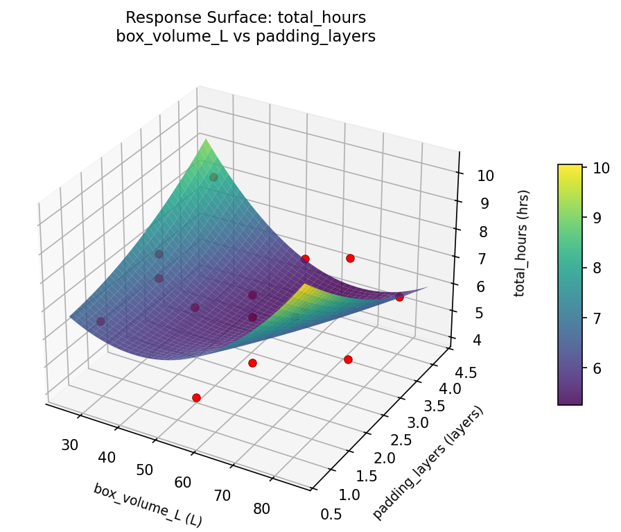
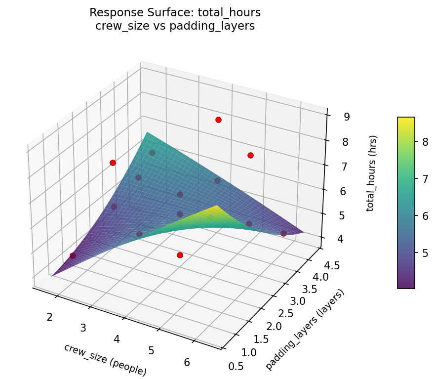
Response Surface Plots
3D surfaces fitted with quadratic RSM. Red dots are observed data points.
breakage pct box volume L vs crew size
breakage pct box volume L vs padding layers
breakage pct crew size vs padding layers
total hours box volume L vs crew size
total hours box volume L vs padding layers
total hours crew size vs padding layers
Multi-Objective Optimization
When responses compete, Derringer–Suich desirability finds the best compromise.
Each response is scaled to a 0–1 desirability, then combined via a weighted geometric mean.
Overall Desirability
D = 0.8397
Per-Response Desirability
| Response | Weight | Desirability | Predicted | Dir |
|---|
total_hours |
1.0 |
|
4.70 0.8409 4.70 hrs |
↓ |
breakage_pct |
1.5 |
|
3.90 0.8388 3.90 % |
↓ |
Recommended Settings
| Factor | Value |
|---|
box_volume_L | 55 L |
crew_size | 4 people |
padding_layers | 2.5 layers |
Source: from observed run #12
Trade-off Summary
Sacrifice = how much worse than single-objective best.
| Response | Predicted | Best Observed | Sacrifice |
|---|
breakage_pct | 3.90 | 3.20 | +0.70 |
Top 3 Runs by Desirability
| Run | D | Factor Settings |
|---|
| #14 | 0.7992 | box_volume_L=30, crew_size=6, padding_layers=2.5 |
| #7 | 0.7480 | box_volume_L=30, crew_size=2, padding_layers=2.5 |
Model Quality
| Response | R² | Type |
|---|
breakage_pct | 0.9429 | quadratic |
Full Multi-Objective Output
============================================================
MULTI-OBJECTIVE OPTIMIZATION
Method: Derringer-Suich Desirability Function
============================================================
Overall desirability: D = 0.8397
Response Weight Desirability Predicted Direction
---------------------------------------------------------------------
total_hours 1.0 0.8409 4.70 hrs ↓
breakage_pct 1.5 0.8388 3.90 % ↓
Recommended settings:
box_volume_L = 55 L
crew_size = 4 people
padding_layers = 2.5 layers
(from observed run #12)
Trade-off summary:
total_hours: 4.70 (best observed: 4.10, sacrifice: +0.60)
breakage_pct: 3.90 (best observed: 3.20, sacrifice: +0.70)
Model quality:
total_hours: R² = 0.0240 (linear)
breakage_pct: R² = 0.9429 (quadratic)
Top 3 observed runs by overall desirability:
1. Run #12 (D=0.8397): box_volume_L=55, crew_size=4, padding_layers=2.5
2. Run #14 (D=0.7992): box_volume_L=30, crew_size=6, padding_layers=2.5
3. Run #7 (D=0.7480): box_volume_L=30, crew_size=2, padding_layers=2.5
Full Analysis Output
=== Main Effects: total_hours ===
Factor Effect Std Error % Contribution
--------------------------------------------------------------
box_volume_L 2.0750 0.3883 61.0%
crew_size 1.1500 0.3883 33.8%
padding_layers 0.1750 0.3883 5.1%
=== ANOVA Table: total_hours ===
Source DF SS MS F p-value
-----------------------------------------------------------------------------
box_volume_L 2 9.2465 4.6233 3.035 0.1045
crew_size 2 2.7547 1.3774 0.904 0.4426
padding_layers 2 0.0622 0.0311 0.020 0.9798
Lack of Fit 6 16.5539 2.7590 1.811 0.3976
Pure Error 2 3.0467 1.5233
Error 8 19.6006 1.5233
Total 14 31.6640 2.2617
=== Summary Statistics: total_hours ===
box_volume_L:
Level N Mean Std Min Max
------------------------------------------------------------
30 4 5.5750 1.0012 4.1000 6.2000
55 7 6.2000 1.5599 4.4000 8.9000
80 4 7.6500 1.2662 5.8000 8.6000
crew_size:
Level N Mean Std Min Max
------------------------------------------------------------
2 4 5.9250 2.1030 4.1000 8.6000
4 7 6.3286 1.0029 4.7000 7.9000
6 4 7.0750 1.7896 5.3000 8.9000
padding_layers:
Level N Mean Std Min Max
------------------------------------------------------------
1 4 6.3250 1.8822 4.4000 8.9000
2.5 7 6.4286 1.7066 4.1000 8.6000
4 4 6.5000 1.0801 5.3000 7.9000
=== Main Effects: breakage_pct ===
Factor Effect Std Error % Contribution
--------------------------------------------------------------
padding_layers 2.0071 0.4237 43.5%
box_volume_L 1.3750 0.4237 29.8%
crew_size 1.2286 0.4237 26.6%
=== ANOVA Table: breakage_pct ===
Source DF SS MS F p-value
-----------------------------------------------------------------------------
box_volume_L 2 3.8482 1.9241 2.337 0.1587
crew_size 2 5.2057 2.6029 3.161 0.0973
padding_layers 2 11.4854 5.7427 6.975 0.0176
Lack of Fit 6 15.5140 2.5857 3.140 0.2611
Pure Error 2 1.6467 0.8233
Error 8 17.1607 0.8233
Total 14 37.7000 2.6929
=== Summary Statistics: breakage_pct ===
box_volume_L:
Level N Mean Std Min Max
------------------------------------------------------------
30 4 6.2500 1.3478 4.9000 7.6000
55 7 5.4286 1.8865 3.2000 8.7000
80 4 4.8750 1.5327 3.2000 6.9000
crew_size:
Level N Mean Std Min Max
------------------------------------------------------------
2 4 6.0000 2.5781 3.2000 8.7000
4 7 4.8714 1.1586 3.2000 6.9000
6 4 6.1000 1.2247 4.5000 7.2000
padding_layers:
Level N Mean Std Min Max
------------------------------------------------------------
1 4 5.0250 0.5500 4.5000 5.8000
2.5 7 4.9429 1.8036 3.2000 7.6000
4 4 6.9500 1.3892 5.3000 8.7000
Optimization Recommendations
=== Optimization: total_hours ===
Direction: minimize
Best observed run: #15
box_volume_L = 80
crew_size = 4
padding_layers = 4
Value: 4.1
RSM Model (linear, R² = 0.1371, Adj R² = -0.0982):
Coefficients:
intercept +6.4200
box_volume_L -0.4000
crew_size +0.6125
padding_layers +0.0875
RSM Model (quadratic, R² = 0.3884, Adj R² = -0.7123):
Coefficients:
intercept +5.8333
box_volume_L -0.4000
crew_size +0.6125
padding_layers +0.0875
box_volume_L*crew_size -0.1250
box_volume_L*padding_layers +0.5250
crew_size*padding_layers -0.4000
box_volume_L^2 -0.5167
crew_size^2 +0.9583
padding_layers^2 +0.6583
Curvature analysis:
crew_size coef=+0.9583 convex (has a minimum)
padding_layers coef=+0.6583 convex (has a minimum)
box_volume_L coef=-0.5167 concave (has a maximum)
Notable interactions:
box_volume_L*padding_layers coef=+0.5250 (synergistic)
crew_size*padding_layers coef=-0.4000 (antagonistic)
Predicted optimum (from linear model, at observed points):
box_volume_L = 30
crew_size = 6
padding_layers = 2.5
Predicted value: 7.4325
Surface optimum (via L-BFGS-B, linear model):
box_volume_L = 80
crew_size = 2
padding_layers = 1
Predicted value: 5.3200
Model quality: Weak fit — consider adding center points or using a different design.
Factor importance:
1. crew_size (effect: 1.6, contribution: 47.2%)
2. box_volume_L (effect: 1.0, contribution: 31.2%)
3. padding_layers (effect: 0.7, contribution: 21.6%)
=== Optimization: breakage_pct ===
Direction: minimize
Best observed run: #7
box_volume_L = 55
crew_size = 4
padding_layers = 2.5
Value: 3.2
RSM Model (linear, R² = 0.1981, Adj R² = -0.0205):
Coefficients:
intercept +5.5000
box_volume_L -0.1250
crew_size +0.9500
padding_layers +0.1250
RSM Model (quadratic, R² = 0.5529, Adj R² = -0.2520):
Coefficients:
intercept +5.7667
box_volume_L -0.1250
crew_size +0.9500
padding_layers +0.1250
box_volume_L*crew_size -0.5500
box_volume_L*padding_layers +1.0500
crew_size*padding_layers +0.3000
box_volume_L^2 +0.8667
crew_size^2 -0.3833
padding_layers^2 -0.9833
Curvature analysis:
padding_layers coef=-0.9833 concave (has a maximum)
box_volume_L coef=+0.8667 convex (has a minimum)
crew_size coef=-0.3833 concave (has a maximum)
Notable interactions:
box_volume_L*padding_layers coef=+1.0500 (synergistic)
box_volume_L*crew_size coef=-0.5500 (antagonistic)
crew_size*padding_layers coef=+0.3000 (synergistic)
Predicted optimum (from linear model, at observed points):
box_volume_L = 55
crew_size = 6
padding_layers = 4
Predicted value: 6.5750
Surface optimum (via L-BFGS-B, linear model):
box_volume_L = 80
crew_size = 2
padding_layers = 1
Predicted value: 4.3000
Model quality: Weak fit — consider adding center points or using a different design.
Factor importance:
1. crew_size (effect: 1.9, contribution: 46.0%)
2. padding_layers (effect: 1.1, contribution: 27.7%)
3. box_volume_L (effect: 1.1, contribution: 26.4%)