Summary
This experiment investigates water well drilling parameters. Central composite design to maximize flow rate and minimize turbidity by tuning drill depth, screen slot size, and gravel pack grade.
The design varies 3 factors: depth m (m), ranging from 15 to 60, screen slot mm (mm), ranging from 0.5 to 2.0, and gravel mm (mm), ranging from 2 to 8. The goal is to optimize 2 responses: flow rate lpm (L/min) (maximize) and turbidity ntu (NTU) (minimize). Fixed conditions held constant across all runs include aquifer = alluvial_sand, casing diam = 150mm.
A Central Composite Design (CCD) was selected to fit a full quadratic response surface model, including curvature and interaction effects. With 3 factors this produces 22 runs including center points and axial (star) points that extend beyond the factorial range.
Quadratic response surface models were fitted to capture potential curvature and factor interactions. The RSM contour plots below visualize how pairs of factors jointly affect each response.
Key Findings
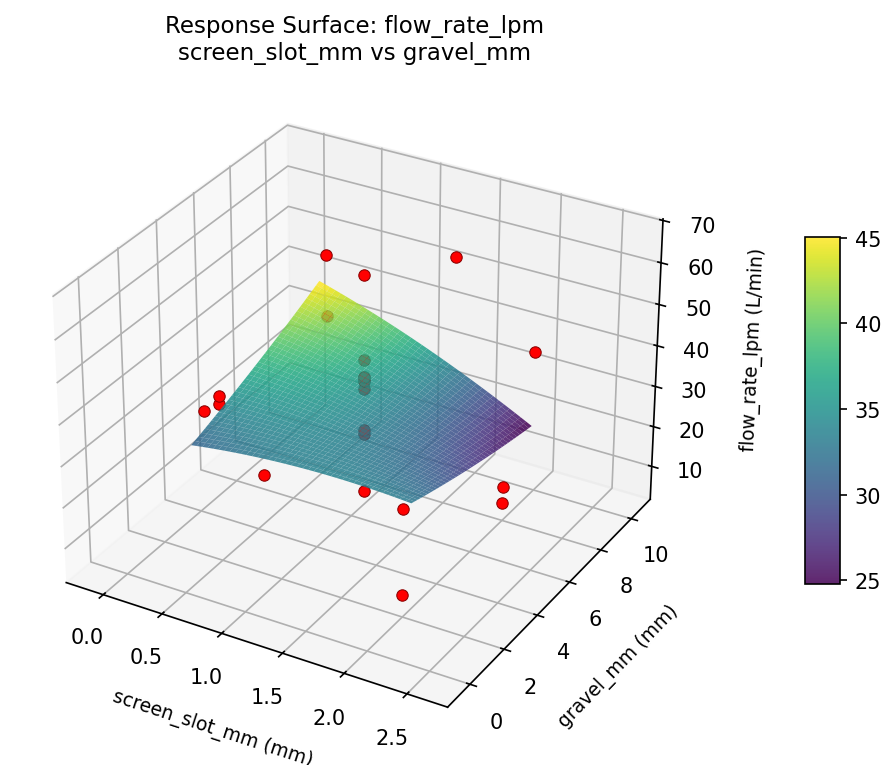
For flow rate lpm, the most influential factors were screen slot mm (49.0%), gravel mm (28.8%), depth m (22.2%). The best observed value was 66.0 (at depth m = 37.5, screen slot mm = 1.25, gravel mm = 5).
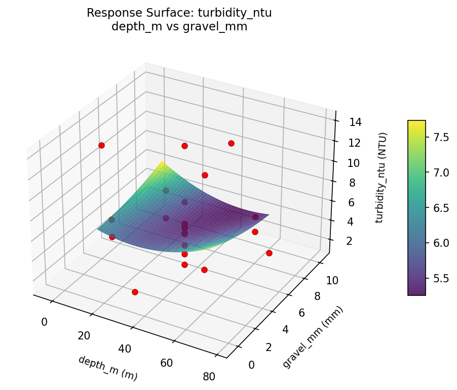
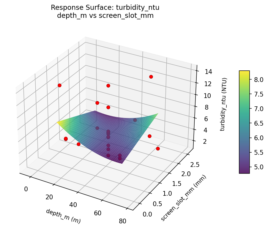
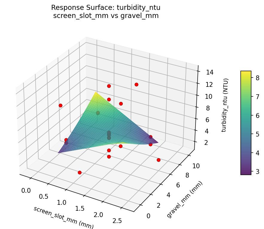
For turbidity ntu, the most influential factors were depth m (34.4%), screen slot mm (33.3%), gravel mm (32.3%). The best observed value was 1.5 (at depth m = 37.5, screen slot mm = 1.25, gravel mm = -0.477226).
Recommended Next Steps
- Run confirmation experiments at the predicted optimal settings to validate the model.
- Consider whether any fixed factors should be varied in a future study.
Experimental Setup
Factors
| Factor | Low | High | Unit |
|---|
depth_m | 15 | 60 | m |
screen_slot_mm | 0.5 | 2.0 | mm |
gravel_mm | 2 | 8 | mm |
Fixed: aquifer = alluvial_sand, casing_diam = 150mm
Responses
| Response | Direction | Unit |
|---|
flow_rate_lpm | ↑ maximize | L/min |
turbidity_ntu | ↓ minimize | NTU |
Configuration
{
"metadata": {
"name": "Water Well Drilling Parameters",
"description": "Central composite design to maximize flow rate and minimize turbidity by tuning drill depth, screen slot size, and gravel pack grade"
},
"factors": [
{
"name": "depth_m",
"levels": [
"15",
"60"
],
"type": "continuous",
"unit": "m"
},
{
"name": "screen_slot_mm",
"levels": [
"0.5",
"2.0"
],
"type": "continuous",
"unit": "mm"
},
{
"name": "gravel_mm",
"levels": [
"2",
"8"
],
"type": "continuous",
"unit": "mm"
}
],
"fixed_factors": {
"aquifer": "alluvial_sand",
"casing_diam": "150mm"
},
"responses": [
{
"name": "flow_rate_lpm",
"optimize": "maximize",
"unit": "L/min"
},
{
"name": "turbidity_ntu",
"optimize": "minimize",
"unit": "NTU"
}
],
"settings": {
"operation": "central_composite",
"test_script": "use_cases/230_well_drilling/sim.sh"
}
}
Experimental Matrix
The Central Composite Design produces 22 runs. Each row is one experiment with specific factor settings.
| Run | depth_m | screen_slot_mm | gravel_mm |
|---|
| 1 | 37.5 | 1.25 | 5 |
| 2 | 60 | 0.5 | 8 |
| 3 | 15 | 2 | 2 |
| 4 | 37.5 | 2.61931 | 5 |
| 5 | 37.5 | 1.25 | 5 |
| 6 | -3.57919 | 1.25 | 5 |
| 7 | 37.5 | 1.25 | -0.477226 |
| 8 | 37.5 | 1.25 | 5 |
| 9 | 60 | 2 | 2 |
| 10 | 78.5792 | 1.25 | 5 |
| 11 | 37.5 | 1.25 | 5 |
| 12 | 37.5 | -0.119306 | 5 |
| 13 | 37.5 | 1.25 | 5 |
| 14 | 15 | 0.5 | 8 |
| 15 | 37.5 | 1.25 | 5 |
| 16 | 60 | 0.5 | 2 |
| 17 | 37.5 | 1.25 | 10.4772 |
| 18 | 60 | 2 | 8 |
| 19 | 37.5 | 1.25 | 5 |
| 20 | 15 | 0.5 | 2 |
| 21 | 15 | 2 | 8 |
| 22 | 37.5 | 1.25 | 5 |
Step-by-Step Workflow
1
Preview the design
$ doe info --config use_cases/230_well_drilling/config.json
2
Generate the runner script
$ doe generate --config use_cases/230_well_drilling/config.json \
--output use_cases/230_well_drilling/results/run.sh --seed 42
3
Execute the experiments
$ bash use_cases/230_well_drilling/results/run.sh
4
Analyze results
$ doe analyze --config use_cases/230_well_drilling/config.json
5
Get optimization recommendations
$ doe optimize --config use_cases/230_well_drilling/config.json
6
Multi-objective optimization
With 2 competing responses, use --multi to find the best compromise via Derringer–Suich desirability.
$ doe optimize --config use_cases/230_well_drilling/config.json --multi
7
Generate the HTML report
$ doe report --config use_cases/230_well_drilling/config.json \
--output use_cases/230_well_drilling/results/report.html
Features Exercised
| Feature | Value |
|---|
| Design type | central_composite |
| Factor types | continuous (all 3) |
| Arg style | double-dash |
| Responses | 2 (flow_rate_lpm ↑, turbidity_ntu ↓) |
| Total runs | 22 |
Analysis Results
Generated from actual experiment runs using the DOE Helper Tool.
Response: flow_rate_lpm
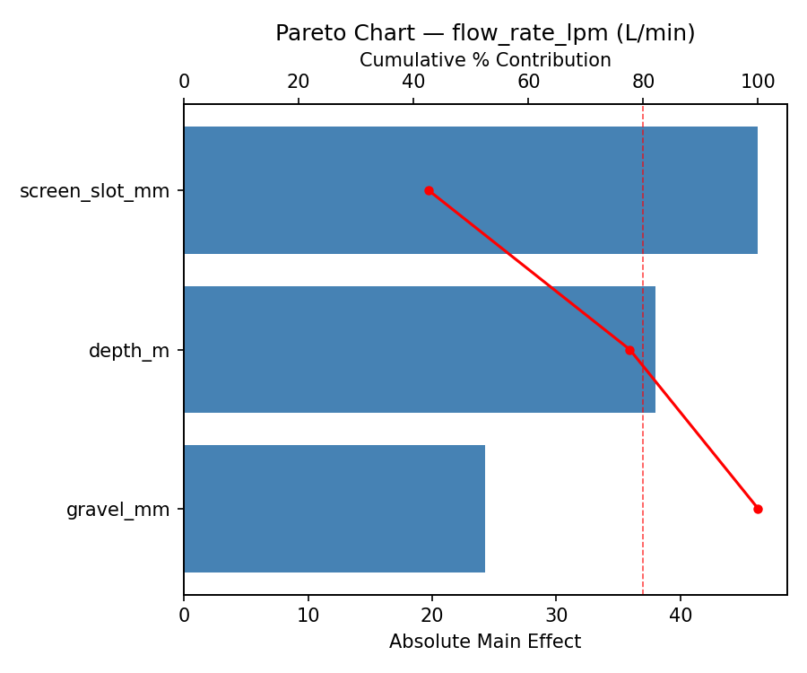
Top factors: screen_slot_mm (49.0%), gravel_mm (28.8%), depth_m (22.2%).
ANOVA
| Source | DF | SS | MS | F | p-value |
|---|
| Source | DF | SS | MS | F | p-value |
| depth_m | 4 | 410.8561 | 102.7140 | 0.381 | 0.8167 |
| screen_slot_mm | 4 | 880.8561 | 220.2140 | 0.818 | 0.5452 |
| gravel_mm | 4 | 756.8561 | 189.2140 | 0.702 | 0.6097 |
| Lack | of | Fit | 2 | 1693.2045 | 846.6023 |
| Pure | Error | 7 | 1885.5000 | | |
| Error | 9 | 3578.7045 | 269.3571 | | |
| Total | 21 | 5627.2727 | 267.9654 | | |
Pareto Chart
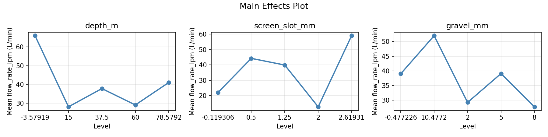
Main Effects Plot
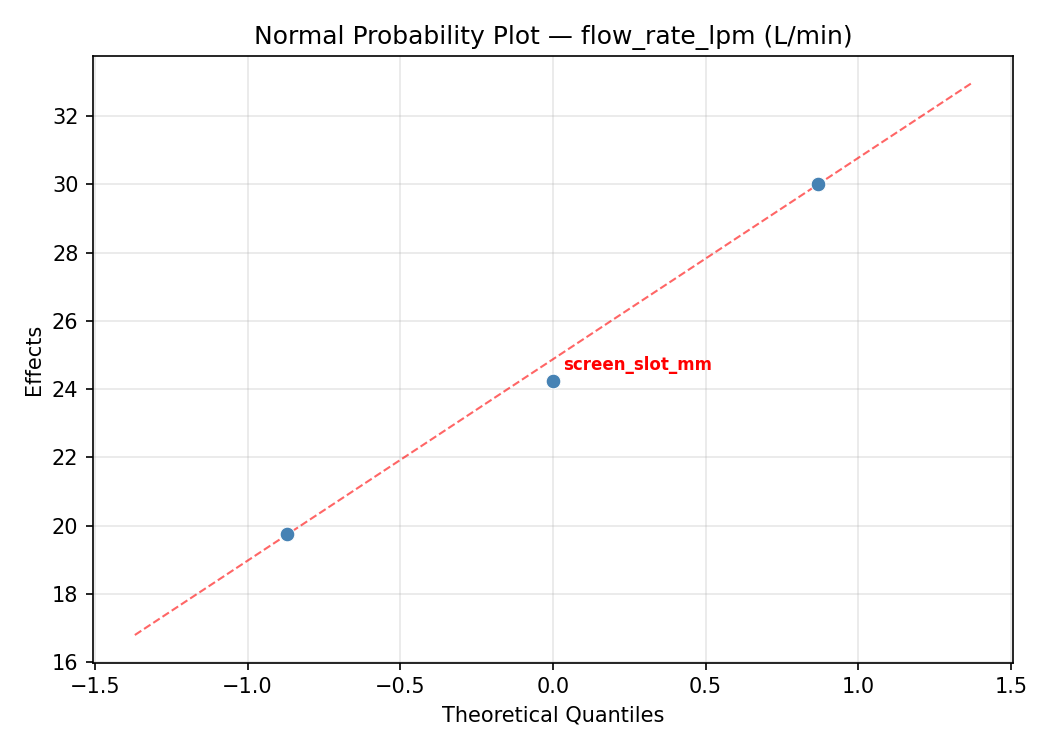
Normal Probability Plot of Effects
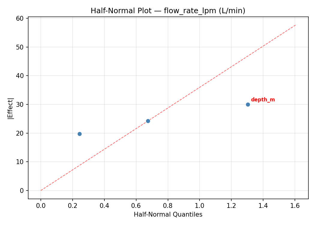
Half-Normal Plot of Effects
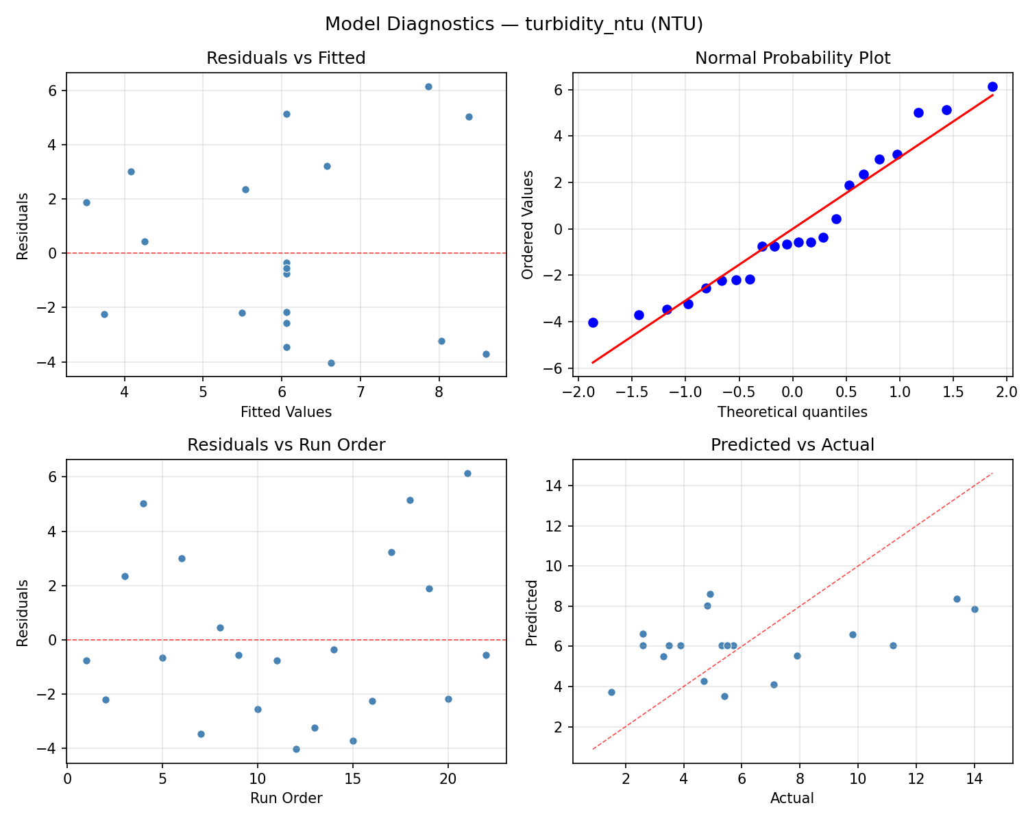
Model Diagnostics
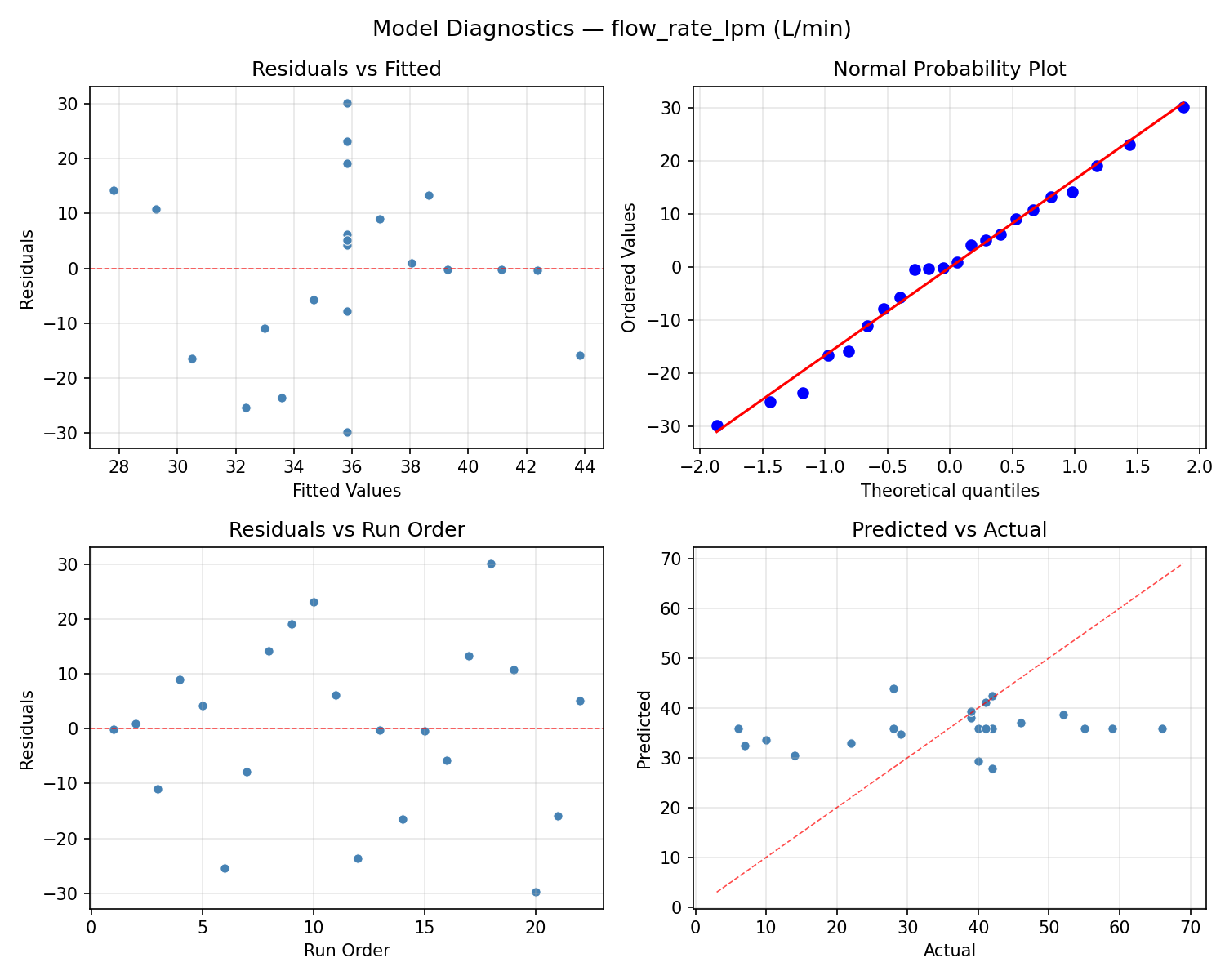
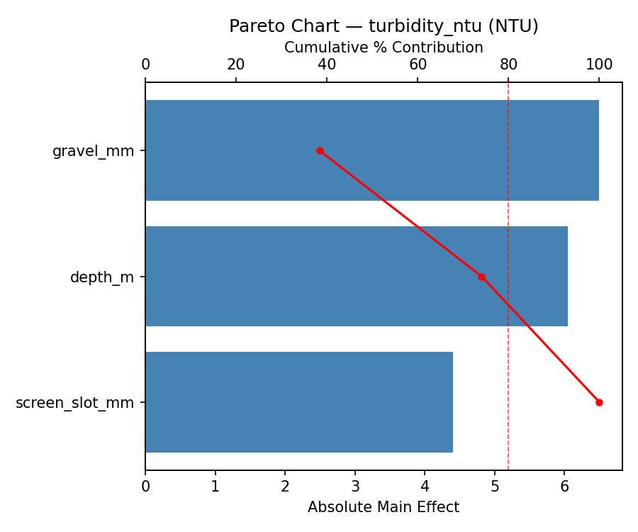
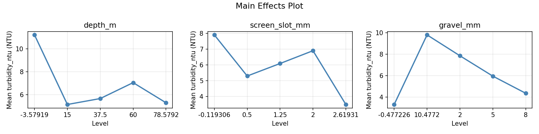
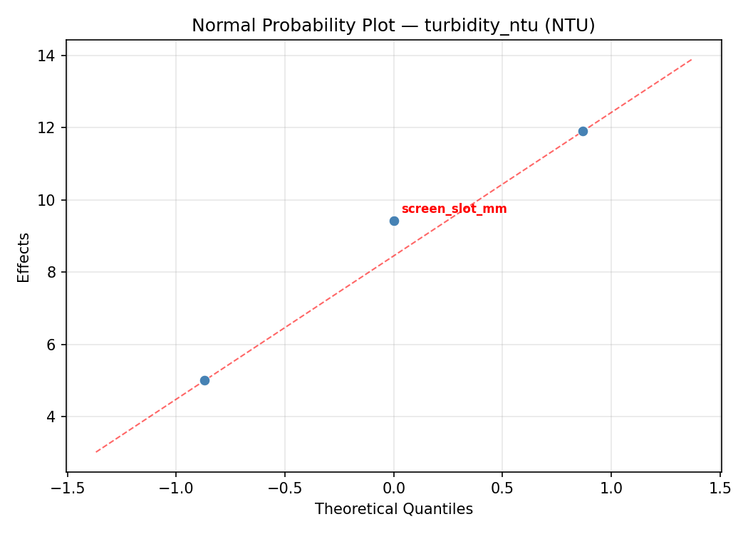
Response: turbidity_ntu
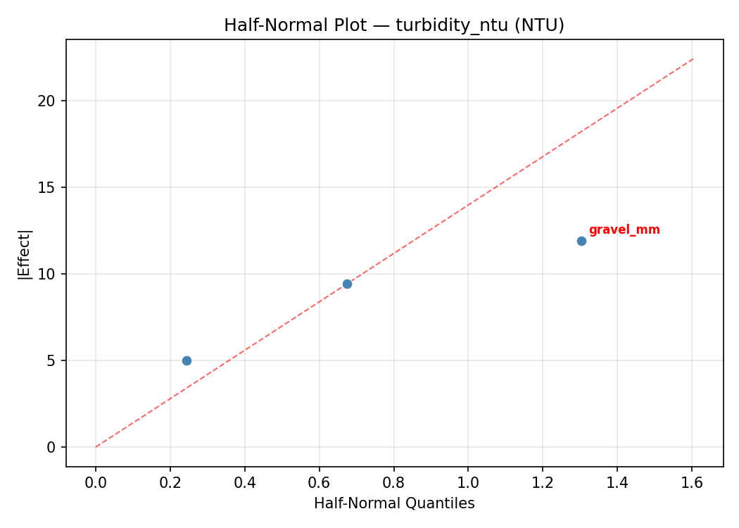
Top factors: depth_m (34.4%), screen_slot_mm (33.3%), gravel_mm (32.3%).
ANOVA
| Source | DF | SS | MS | F | p-value |
|---|
| Source | DF | SS | MS | F | p-value |
| depth_m | 4 | 20.9157 | 5.2289 | 0.299 | 0.8717 |
| screen_slot_mm | 4 | 32.4090 | 8.1023 | 0.463 | 0.7619 |
| gravel_mm | 4 | 43.8132 | 10.9533 | 0.626 | 0.6562 |
| Lack | of | Fit | 2 | 13.2166 | 6.6083 |
| Pure | Error | 7 | 122.5788 | | |
| Error | 9 | 135.7953 | 17.5113 | | |
| Total | 21 | 232.9332 | 11.0921 | | |
Pareto Chart
Main Effects Plot
Normal Probability Plot of Effects
Half-Normal Plot of Effects
Model Diagnostics
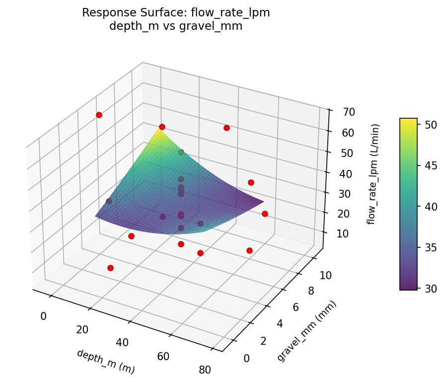
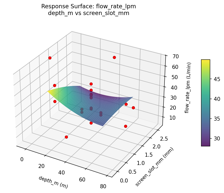
Response Surface Plots
3D surfaces fitted with quadratic RSM. Red dots are observed data points.
flow rate lpm depth m vs gravel mm
flow rate lpm depth m vs screen slot mm
flow rate lpm screen slot mm vs gravel mm
turbidity ntu depth m vs gravel mm
turbidity ntu depth m vs screen slot mm
turbidity ntu screen slot mm vs gravel mm
Multi-Objective Optimization
When responses compete, Derringer–Suich desirability finds the best compromise.
Each response is scaled to a 0–1 desirability, then combined via a weighted geometric mean.
Overall Desirability
D = 0.8325
Per-Response Desirability
| Response | Weight | Desirability | Predicted | Dir |
|---|
flow_rate_lpm |
1.5 |
|
59.00 0.8485 59.00 L/min |
↑ |
turbidity_ntu |
1.0 |
|
3.50 0.8091 3.50 NTU |
↓ |
Recommended Settings
| Factor | Value |
|---|
depth_m | 78.5792 m |
screen_slot_mm | 1.25 mm |
gravel_mm | 5 mm |
Source: from observed run #10
Trade-off Summary
Sacrifice = how much worse than single-objective best.
| Response | Predicted | Best Observed | Sacrifice |
|---|
turbidity_ntu | 3.50 | 1.50 | +2.00 |
Top 3 Runs by Desirability
| Run | D | Factor Settings |
|---|
| #9 | 0.7356 | depth_m=37.5, screen_slot_mm=1.25, gravel_mm=-0.477226 |
| #2 | 0.6432 | depth_m=15, screen_slot_mm=0.5, gravel_mm=2 |
Model Quality
| Response | R² | Type |
|---|
turbidity_ntu | 0.0841 | linear |
Full Multi-Objective Output
============================================================
MULTI-OBJECTIVE OPTIMIZATION
Method: Derringer-Suich Desirability Function
============================================================
Overall desirability: D = 0.8325
Response Weight Desirability Predicted Direction
---------------------------------------------------------------------
flow_rate_lpm 1.5 0.8485 59.00 L/min ↑
turbidity_ntu 1.0 0.8091 3.50 NTU ↓
Recommended settings:
depth_m = 78.5792 m
screen_slot_mm = 1.25 mm
gravel_mm = 5 mm
(from observed run #10)
Trade-off summary:
flow_rate_lpm: 59.00 (best observed: 66.00, sacrifice: +7.00)
turbidity_ntu: 3.50 (best observed: 1.50, sacrifice: +2.00)
Model quality:
flow_rate_lpm: R² = 0.4609 (quadratic)
turbidity_ntu: R² = 0.0841 (linear)
Top 3 observed runs by overall desirability:
1. Run #10 (D=0.8325): depth_m=78.5792, screen_slot_mm=1.25, gravel_mm=5
2. Run #9 (D=0.7356): depth_m=37.5, screen_slot_mm=1.25, gravel_mm=-0.477226
3. Run #2 (D=0.6432): depth_m=15, screen_slot_mm=0.5, gravel_mm=2
Full Analysis Output
=== Main Effects: flow_rate_lpm ===
Factor Effect Std Error % Contribution
--------------------------------------------------------------
screen_slot_mm 29.7500 3.4900 49.0%
gravel_mm 17.5000 3.4900 28.8%
depth_m 13.5000 3.4900 22.2%
=== ANOVA Table: flow_rate_lpm ===
Source DF SS MS F p-value
-----------------------------------------------------------------------------
depth_m 4 410.8561 102.7140 0.381 0.8167
screen_slot_mm 4 880.8561 220.2140 0.818 0.5452
gravel_mm 4 756.8561 189.2140 0.702 0.6097
Lack of Fit 2 1693.2045 846.6023 3.143 0.1062
Pure Error 7 1885.5000 269.3571
Error 9 3578.7045 269.3571
Total 21 5627.2727 267.9654
=== Summary Statistics: flow_rate_lpm ===
depth_m:
Level N Mean Std Min Max
------------------------------------------------------------
-3.57919 1 42.0000 0.0000 42.0000 42.0000
15 4 28.5000 16.0520 6.0000 41.0000
37.5 12 38.6667 14.2659 10.0000 59.0000
60 4 32.2500 27.1093 7.0000 66.0000
78.5792 1 39.0000 0.0000 39.0000 39.0000
screen_slot_mm:
Level N Mean Std Min Max
------------------------------------------------------------
-0.119306 1 42.0000 0.0000 42.0000 42.0000
0.5 4 25.2500 17.2892 7.0000 41.0000
1.25 12 37.3333 13.3167 10.0000 59.0000
2 4 35.5000 25.1595 6.0000 66.0000
2.61931 1 55.0000 0.0000 55.0000 55.0000
gravel_mm:
Level N Mean Std Min Max
------------------------------------------------------------
-0.477226 1 40.0000 0.0000 40.0000 40.0000
10.4772 1 41.0000 0.0000 41.0000 41.0000
2 4 23.5000 19.6723 6.0000 42.0000
5 12 38.6667 14.2786 10.0000 59.0000
8 4 37.2500 22.1115 14.0000 66.0000
=== Main Effects: turbidity_ntu ===
Factor Effect Std Error % Contribution
--------------------------------------------------------------
depth_m 4.0250 0.7101 34.4%
screen_slot_mm 3.9000 0.7101 33.3%
gravel_mm 3.7750 0.7101 32.3%
=== ANOVA Table: turbidity_ntu ===
Source DF SS MS F p-value
-----------------------------------------------------------------------------
depth_m 4 20.9157 5.2289 0.299 0.8717
screen_slot_mm 4 32.4090 8.1023 0.463 0.7619
gravel_mm 4 43.8132 10.9533 0.626 0.6562
Lack of Fit 2 13.2166 6.6083 0.377 0.6988
Pure Error 7 122.5788 17.5113
Error 9 135.7953 17.5113
Total 21 232.9332 11.0921
=== Summary Statistics: turbidity_ntu ===
depth_m:
Level N Mean Std Min Max
------------------------------------------------------------
-3.57919 1 4.9000 0.0000 4.9000 4.9000
15 4 7.0000 4.7025 3.9000 14.0000
37.5 12 5.6500 3.3557 1.5000 13.4000
60 4 7.3250 2.6961 5.3000 11.2000
78.5792 1 3.3000 0.0000 3.3000 3.3000
screen_slot_mm:
Level N Mean Std Min Max
------------------------------------------------------------
-0.119306 1 4.7000 0.0000 4.7000 4.7000
0.5 4 5.7250 0.9878 4.8000 7.1000
1.25 12 5.4833 3.4205 1.5000 13.4000
2 4 8.6000 4.7924 3.9000 14.0000
2.61931 1 5.5000 0.0000 5.5000 5.5000
gravel_mm:
Level N Mean Std Min Max
------------------------------------------------------------
-0.477226 1 5.4000 0.0000 5.4000 5.4000
10.4772 1 5.5000 0.0000 5.5000 5.5000
2 4 5.2750 1.3475 3.9000 7.1000
5 12 5.4250 3.4280 1.5000 13.4000
8 4 9.0500 4.2587 5.3000 14.0000
Optimization Recommendations
=== Optimization: flow_rate_lpm ===
Direction: maximize
Best observed run: #18
depth_m = 37.5
screen_slot_mm = 1.25
gravel_mm = 5
Value: 66.0
RSM Model (linear, R² = 0.0887, Adj R² = -0.0631):
Coefficients:
intercept +35.8182
depth_m -4.4824
screen_slot_mm +2.6859
gravel_mm +2.5966
RSM Model (quadratic, R² = 0.4361, Adj R² = 0.0132):
Coefficients:
intercept +37.4761
depth_m -4.4824
screen_slot_mm +2.6860
gravel_mm +2.5966
depth_m*screen_slot_mm +5.2500
depth_m*gravel_mm -5.7500
screen_slot_mm*gravel_mm +1.5000
depth_m^2 +4.1210
screen_slot_mm^2 -6.9789
gravel_mm^2 +0.3711
Curvature analysis:
screen_slot_mm coef=-6.9789 concave (has a maximum)
depth_m coef=+4.1210 convex (has a minimum)
gravel_mm coef=+0.3711 convex (has a minimum)
Notable interactions:
depth_m*gravel_mm coef=-5.7500 (antagonistic)
depth_m*screen_slot_mm coef=+5.2500 (synergistic)
screen_slot_mm*gravel_mm coef=+1.5000 (synergistic)
Predicted optimum (from quadratic model, at observed points):
depth_m = -3.57919
screen_slot_mm = 1.25
gravel_mm = 5
Predicted value: 59.3967
Surface optimum (via L-BFGS-B, quadratic model):
depth_m = 15
screen_slot_mm = 1.19283
gravel_mm = 8
Predicted value: 54.8378
Model quality: Weak fit — consider adding center points or using a different design.
Factor importance:
1. screen_slot_mm (effect: 39.2, contribution: 52.3%)
2. depth_m (effect: 24.0, contribution: 32.0%)
3. gravel_mm (effect: 11.8, contribution: 15.7%)
=== Optimization: turbidity_ntu ===
Direction: minimize
Best observed run: #16
depth_m = 37.5
screen_slot_mm = 1.25
gravel_mm = -0.477226
Value: 1.5
RSM Model (linear, R² = 0.0424, Adj R² = -0.1172):
Coefficients:
intercept +6.0591
depth_m +0.6236
screen_slot_mm -0.5241
gravel_mm -0.1009
RSM Model (quadratic, R² = 0.3244, Adj R² = -0.1823):
Coefficients:
intercept +7.9301
depth_m +0.6236
screen_slot_mm -0.5241
gravel_mm -0.1009
depth_m*screen_slot_mm +0.1250
depth_m*gravel_mm -0.8000
screen_slot_mm*gravel_mm +0.2250
depth_m^2 -0.2905
screen_slot_mm^2 -1.0555
gravel_mm^2 -1.4605
Curvature analysis:
gravel_mm coef=-1.4605 concave (has a maximum)
screen_slot_mm coef=-1.0555 concave (has a maximum)
depth_m coef=-0.2905 concave (has a maximum)
Notable interactions:
depth_m*gravel_mm coef=-0.8000 (antagonistic)
Predicted optimum (from linear model, at observed points):
depth_m = 60
screen_slot_mm = 0.5
gravel_mm = 2
Predicted value: 7.3076
Surface optimum (via L-BFGS-B, linear model):
depth_m = 15
screen_slot_mm = 2
gravel_mm = 8
Predicted value: 4.8105
Model quality: Weak fit — consider adding center points or using a different design.
Factor importance:
1. gravel_mm (effect: 5.8, contribution: 41.5%)
2. depth_m (effect: 5.0, contribution: 35.7%)
3. screen_slot_mm (effect: 3.2, contribution: 22.8%)