Summary
This experiment investigates seismograph network placement. Full factorial of station spacing, depth of burial, sampling rate, and filter bandwidth to maximize event detection and minimize false triggers.
The design varies 4 factors: spacing km (km), ranging from 5 to 25, burial m (m), ranging from 0 to 3, sample hz (Hz), ranging from 40 to 200, and filter hz (Hz), ranging from 0.5 to 10. The goal is to optimize 2 responses: detection pct (%) (maximize) and false trigger day (per_day) (minimize). Fixed conditions held constant across all runs include sensor = broadband, network size = 8_stations.
A full factorial design was used to explore all 16 possible combinations of the 4 factors at two levels. This guarantees that every main effect and interaction can be estimated independently, at the cost of a larger experiment (16 runs).
Quadratic response surface models were fitted to capture potential curvature and factor interactions. The RSM contour plots below visualize how pairs of factors jointly affect each response.
Key Findings
For detection pct, the most influential factors were sample hz (55.4%), filter hz (33.7%), burial m (8.4%). The best observed value was 100.0 (at spacing km = 5, burial m = 3, sample hz = 200).
For false trigger day, the most influential factors were filter hz (34.1%), spacing km (29.4%), burial m (22.7%). The best observed value was -0.0 (at spacing km = 25, burial m = 3, sample hz = 200).
Recommended Next Steps
- Consider whether any fixed factors should be varied in a future study.
Experimental Setup
Factors
| Factor | Low | High | Unit |
|---|
spacing_km | 5 | 25 | km |
burial_m | 0 | 3 | m |
sample_hz | 40 | 200 | Hz |
filter_hz | 0.5 | 10 | Hz |
Fixed: sensor = broadband, network_size = 8_stations
Responses
| Response | Direction | Unit |
|---|
detection_pct | ↑ maximize | % |
false_trigger_day | ↓ minimize | per_day |
Configuration
{
"metadata": {
"name": "Seismograph Network Placement",
"description": "Full factorial of station spacing, depth of burial, sampling rate, and filter bandwidth to maximize event detection and minimize false triggers"
},
"factors": [
{
"name": "spacing_km",
"levels": [
"5",
"25"
],
"type": "continuous",
"unit": "km"
},
{
"name": "burial_m",
"levels": [
"0",
"3"
],
"type": "continuous",
"unit": "m"
},
{
"name": "sample_hz",
"levels": [
"40",
"200"
],
"type": "continuous",
"unit": "Hz"
},
{
"name": "filter_hz",
"levels": [
"0.5",
"10"
],
"type": "continuous",
"unit": "Hz"
}
],
"fixed_factors": {
"sensor": "broadband",
"network_size": "8_stations"
},
"responses": [
{
"name": "detection_pct",
"optimize": "maximize",
"unit": "%"
},
{
"name": "false_trigger_day",
"optimize": "minimize",
"unit": "per_day"
}
],
"settings": {
"operation": "full_factorial",
"test_script": "use_cases/232_seismograph_placement/sim.sh"
}
}
Experimental Matrix
The Full Factorial Design produces 16 runs. Each row is one experiment with specific factor settings.
| Run | spacing_km | burial_m | sample_hz | filter_hz |
|---|
| 1 | 5 | 3 | 200 | 10 |
| 2 | 25 | 0 | 40 | 10 |
| 3 | 5 | 3 | 40 | 10 |
| 4 | 5 | 3 | 200 | 0.5 |
| 5 | 25 | 3 | 200 | 0.5 |
| 6 | 25 | 0 | 200 | 0.5 |
| 7 | 25 | 3 | 40 | 0.5 |
| 8 | 25 | 0 | 40 | 0.5 |
| 9 | 5 | 0 | 40 | 10 |
| 10 | 5 | 0 | 200 | 0.5 |
| 11 | 25 | 3 | 40 | 10 |
| 12 | 25 | 3 | 200 | 10 |
| 13 | 5 | 3 | 40 | 0.5 |
| 14 | 25 | 0 | 200 | 10 |
| 15 | 5 | 0 | 40 | 0.5 |
| 16 | 5 | 0 | 200 | 10 |
Step-by-Step Workflow
1
Preview the design
$ doe info --config use_cases/232_seismograph_placement/config.json
2
Generate the runner script
$ doe generate --config use_cases/232_seismograph_placement/config.json \
--output use_cases/232_seismograph_placement/results/run.sh --seed 42
3
Execute the experiments
$ bash use_cases/232_seismograph_placement/results/run.sh
4
Analyze results
$ doe analyze --config use_cases/232_seismograph_placement/config.json
5
Get optimization recommendations
$ doe optimize --config use_cases/232_seismograph_placement/config.json
6
Multi-objective optimization
With 2 competing responses, use --multi to find the best compromise via Derringer–Suich desirability.
$ doe optimize --config use_cases/232_seismograph_placement/config.json --multi
7
Generate the HTML report
$ doe report --config use_cases/232_seismograph_placement/config.json \
--output use_cases/232_seismograph_placement/results/report.html
Features Exercised
| Feature | Value |
|---|
| Design type | full_factorial |
| Factor types | continuous (all 4) |
| Arg style | double-dash |
| Responses | 2 (detection_pct ↑, false_trigger_day ↓) |
| Total runs | 16 |
Analysis Results
Generated from actual experiment runs using the DOE Helper Tool.
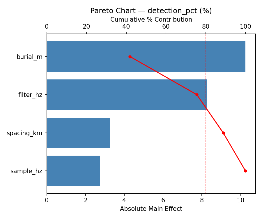
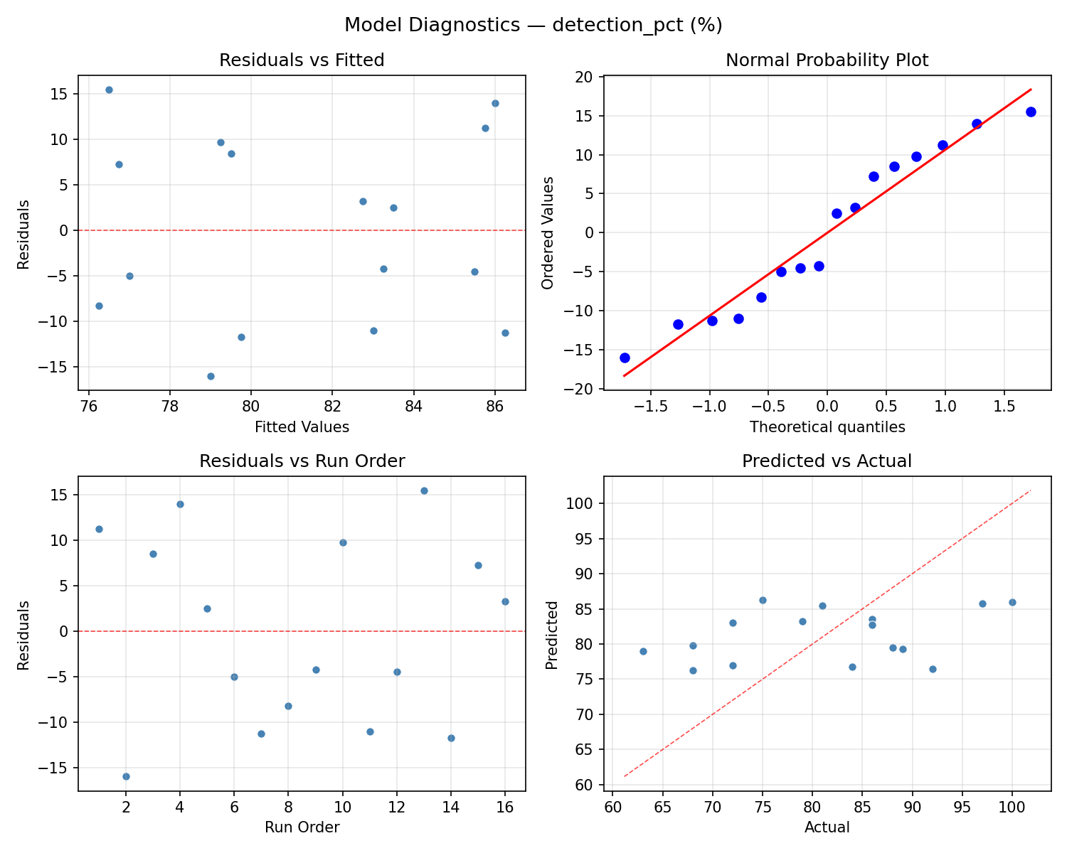
Response: detection_pct
Top factors: sample_hz (55.4%), filter_hz (33.7%), burial_m (8.4%).
ANOVA
| Source | DF | SS | MS | F | p-value |
|---|
| Source | DF | SS | MS | F | p-value |
| spacing_km | 1 | 1.0000 | 1.0000 | 0.014 | 0.9117 |
| burial_m | 1 | 12.2500 | 12.2500 | 0.166 | 0.7002 |
| sample_hz | 1 | 529.0000 | 529.0000 | 7.188 | 0.0438 |
| filter_hz | 1 | 196.0000 | 196.0000 | 2.663 | 0.1636 |
| spacing_km*burial_m | 1 | 12.2500 | 12.2500 | 0.166 | 0.7002 |
| spacing_km*sample_hz | 1 | 196.0000 | 196.0000 | 2.663 | 0.1636 |
| spacing_km*filter_hz | 1 | 324.0000 | 324.0000 | 4.402 | 0.0900 |
| burial_m*sample_hz | 1 | 42.2500 | 42.2500 | 0.574 | 0.4828 |
| burial_m*filter_hz | 1 | 56.2500 | 56.2500 | 0.764 | 0.4220 |
| sample_hz*filter_hz | 1 | 36.0000 | 36.0000 | 0.489 | 0.5155 |
| Error | 5 | 368.0000 | 73.6000 | | |
| Total | 15 | 1773.0000 | 118.2000 | | |
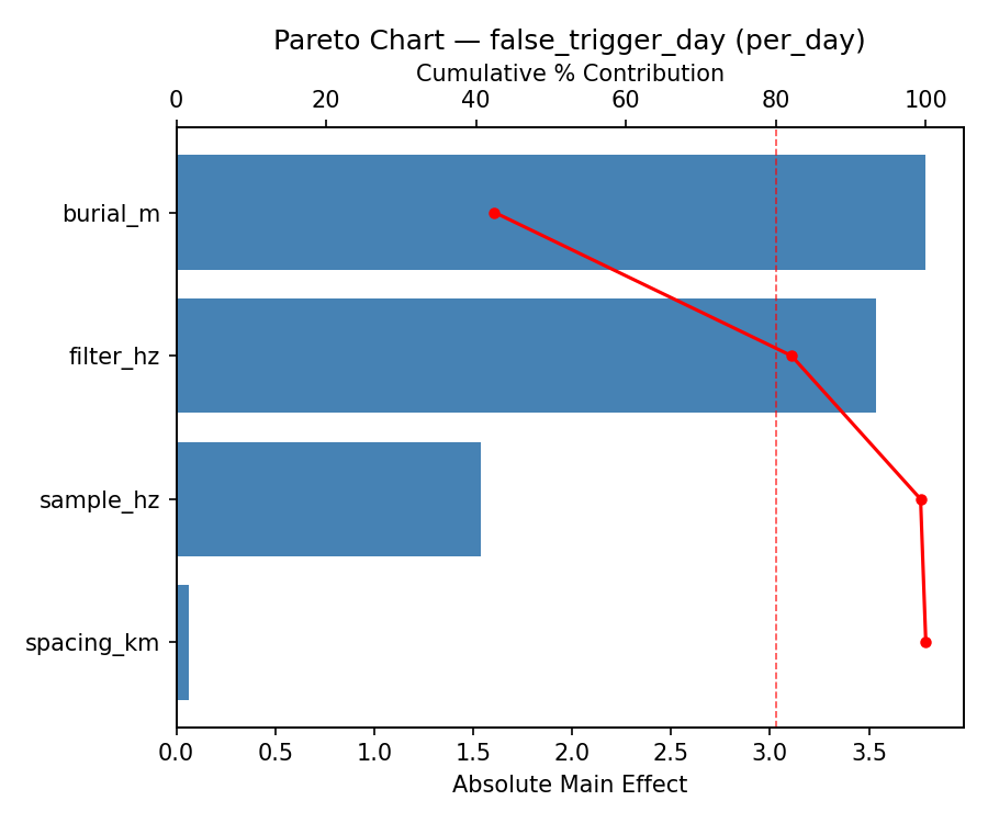
Pareto Chart
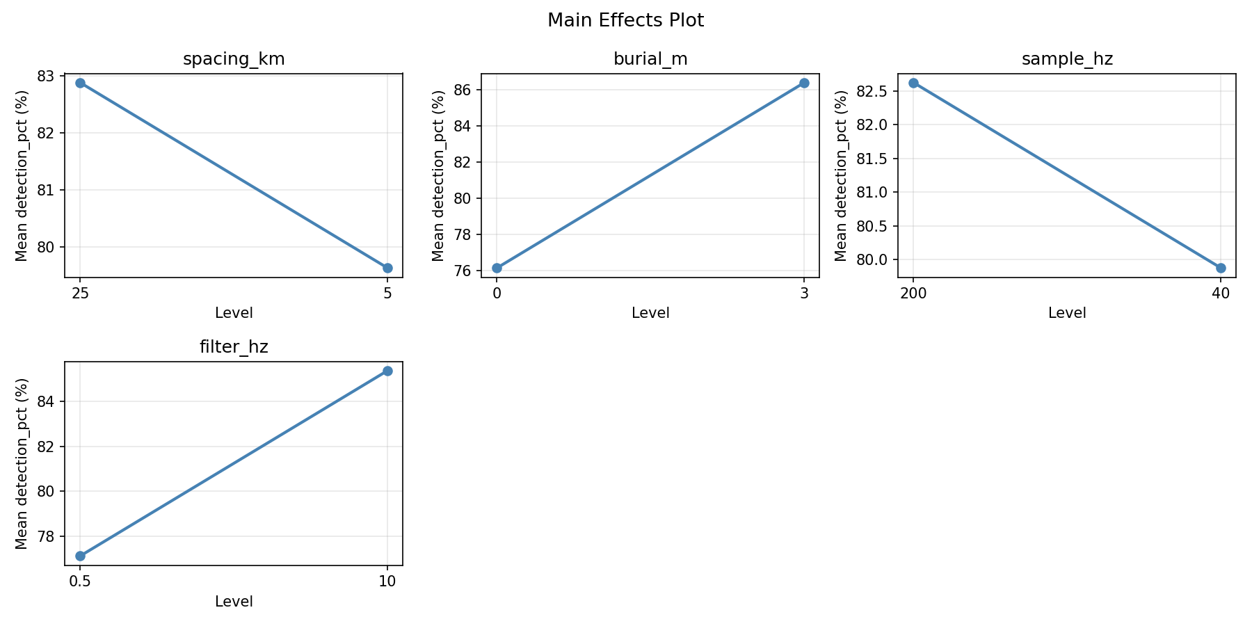
Main Effects Plot
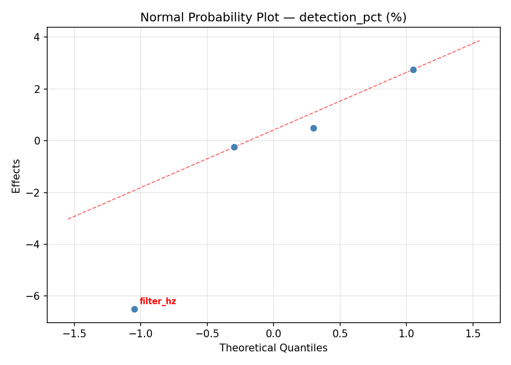
Normal Probability Plot of Effects
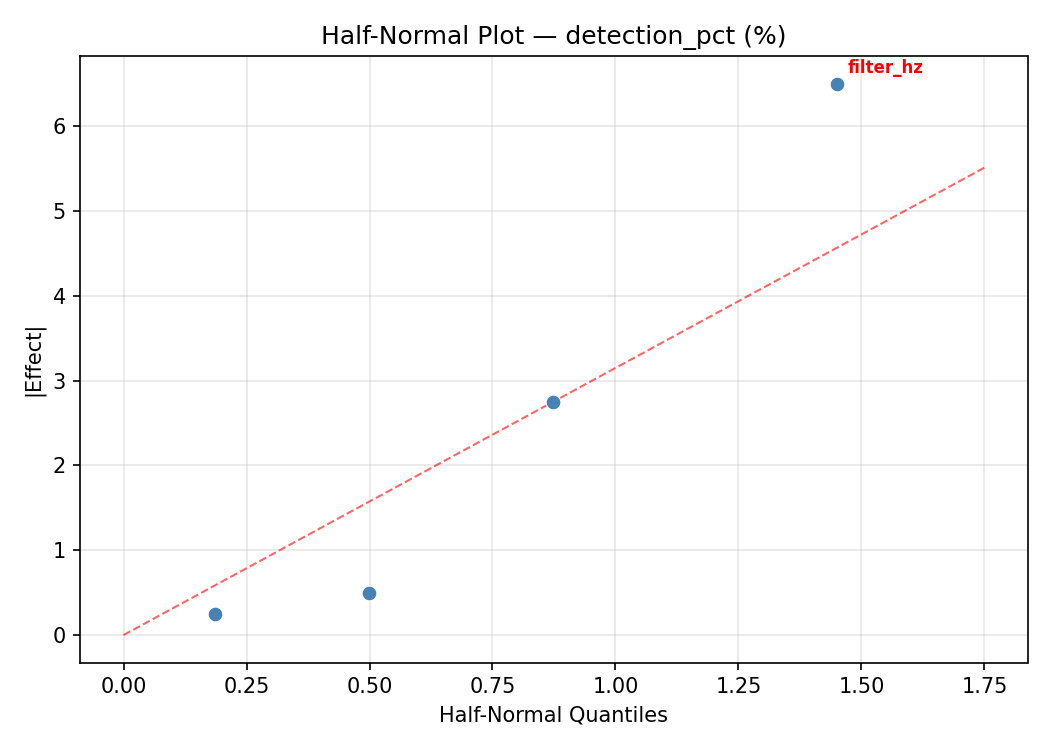
Half-Normal Plot of Effects
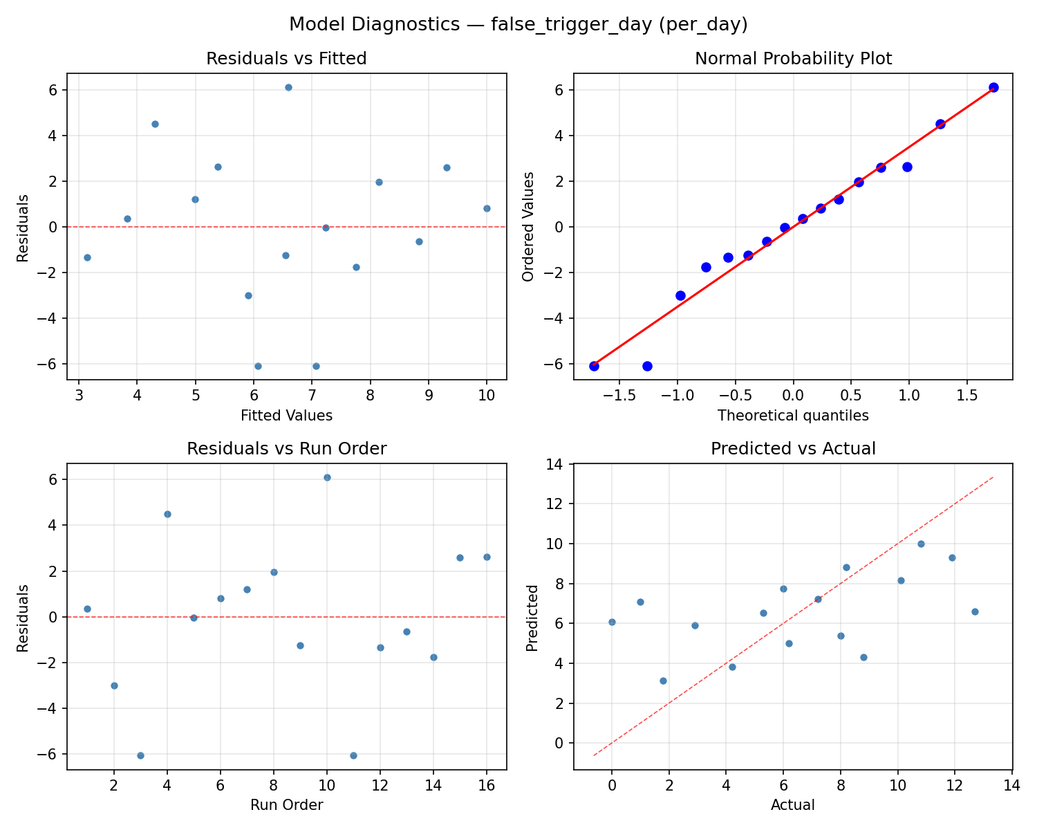
Model Diagnostics
Response: false_trigger_day
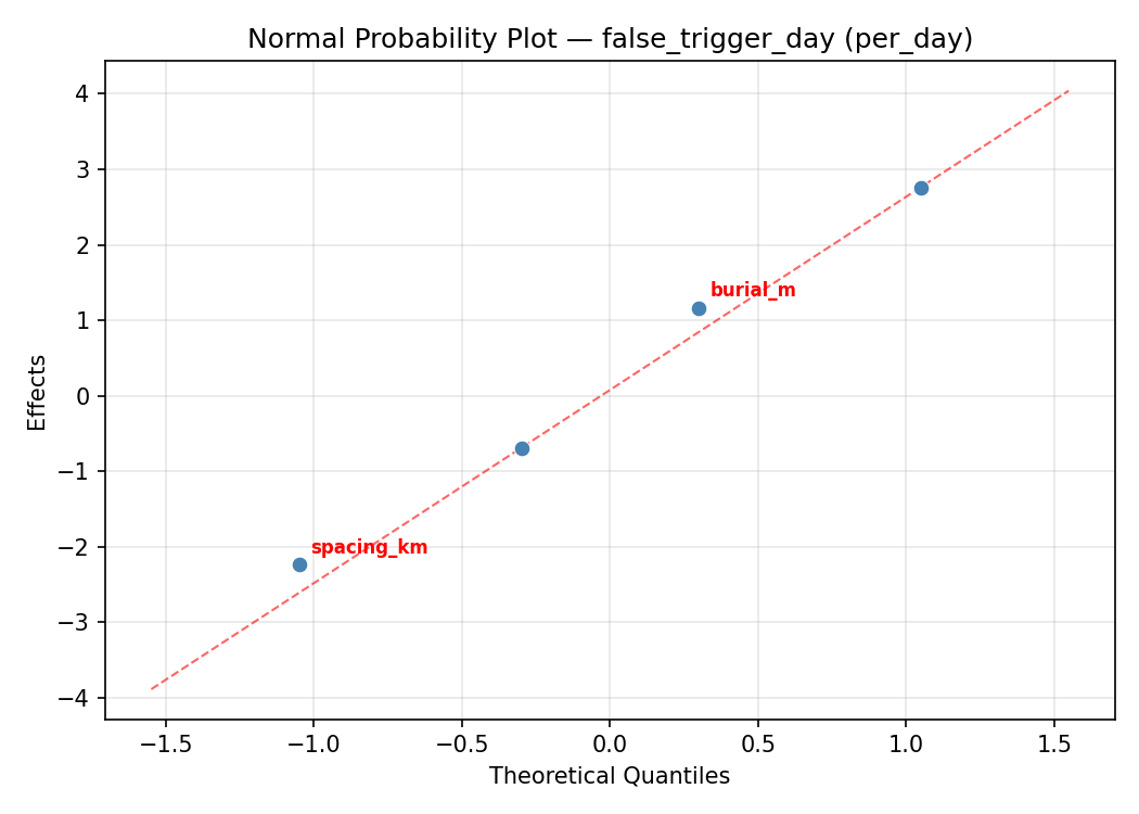
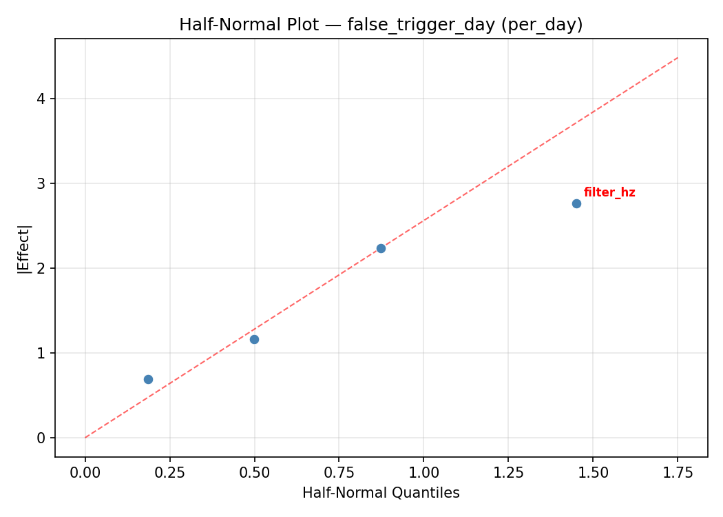
Top factors: filter_hz (34.1%), spacing_km (29.4%), burial_m (22.7%).
ANOVA
| Source | DF | SS | MS | F | p-value |
|---|
| Source | DF | SS | MS | F | p-value |
| spacing_km | 1 | 7.9806 | 7.9806 | 0.555 | 0.4897 |
| burial_m | 1 | 4.7306 | 4.7306 | 0.329 | 0.5910 |
| sample_hz | 1 | 1.7556 | 1.7556 | 0.122 | 0.7409 |
| filter_hz | 1 | 10.7256 | 10.7256 | 0.746 | 0.4271 |
| spacing_km*burial_m | 1 | 1.6256 | 1.6256 | 0.113 | 0.7503 |
| spacing_km*sample_hz | 1 | 5.4056 | 5.4056 | 0.376 | 0.5665 |
| spacing_km*filter_hz | 1 | 0.0756 | 0.0756 | 0.005 | 0.9450 |
| burial_m*sample_hz | 1 | 11.3906 | 11.3906 | 0.793 | 0.4141 |
| burial_m*filter_hz | 1 | 72.6756 | 72.6756 | 5.058 | 0.0744 |
| sample_hz*filter_hz | 1 | 36.3006 | 36.3006 | 2.526 | 0.1728 |
| Error | 5 | 71.8481 | 14.3696 | | |
| Total | 15 | 224.5144 | 14.9676 | | |
Pareto Chart
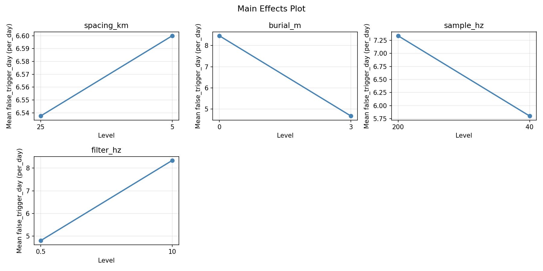
Main Effects Plot
Normal Probability Plot of Effects
Half-Normal Plot of Effects
Model Diagnostics
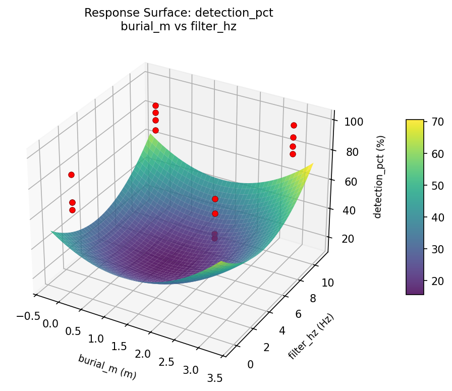
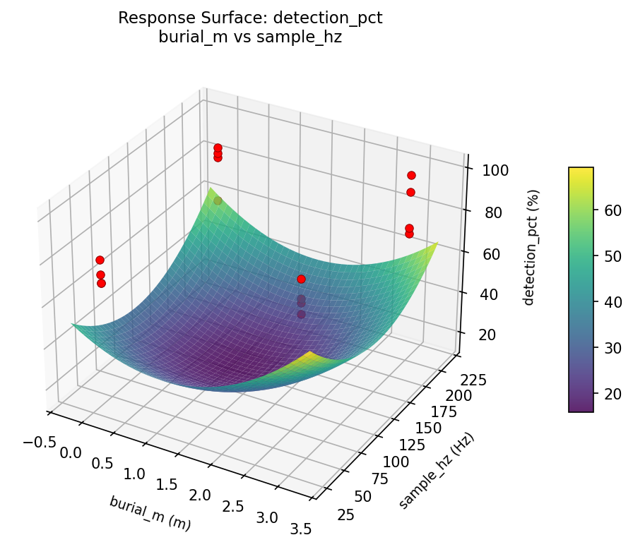
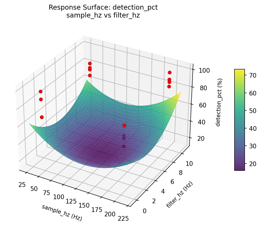
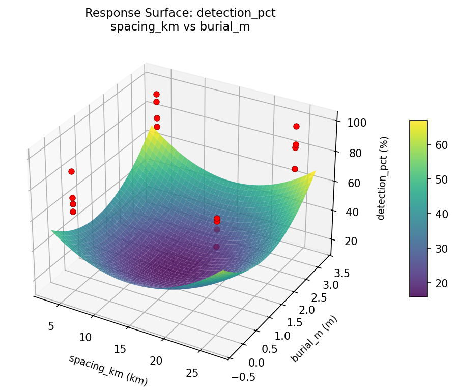
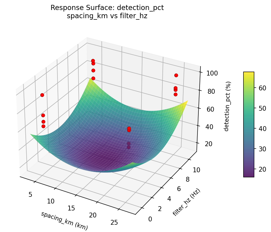
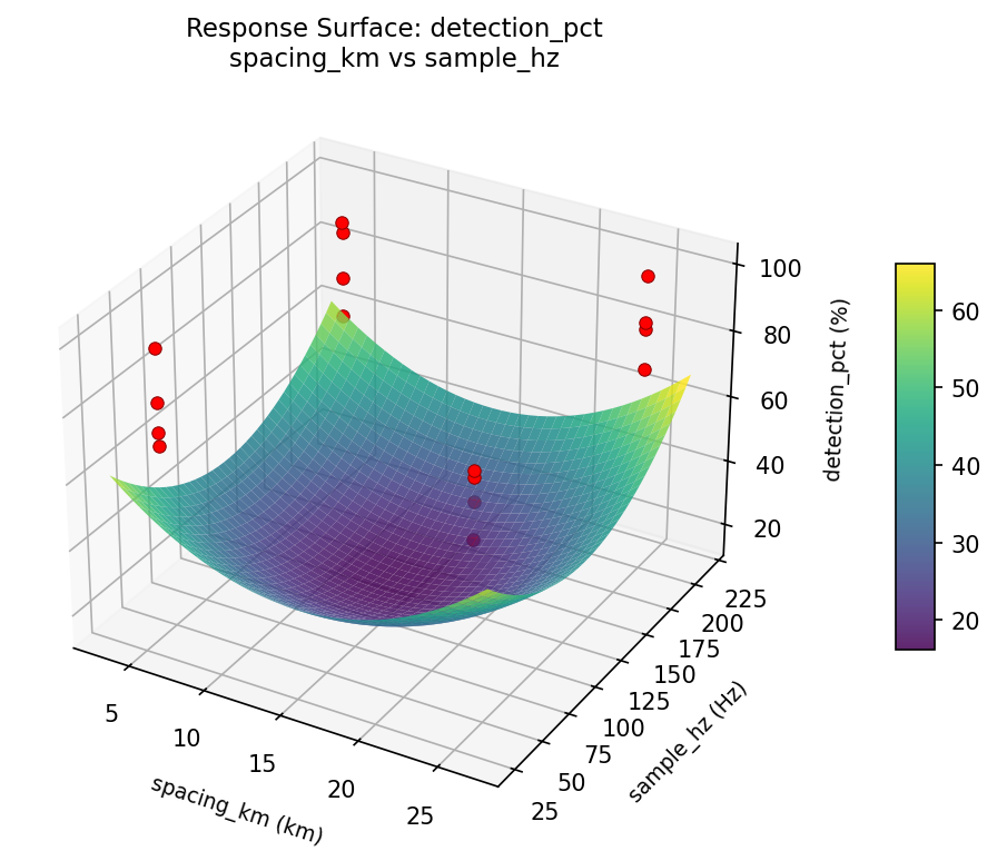
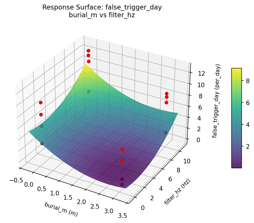
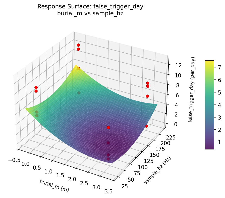
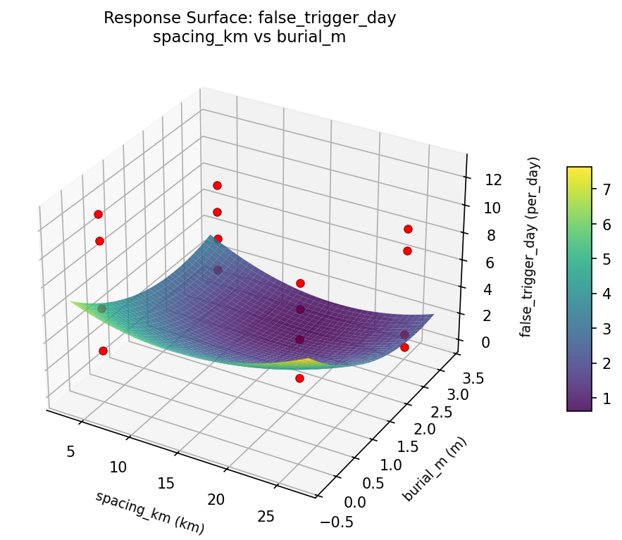
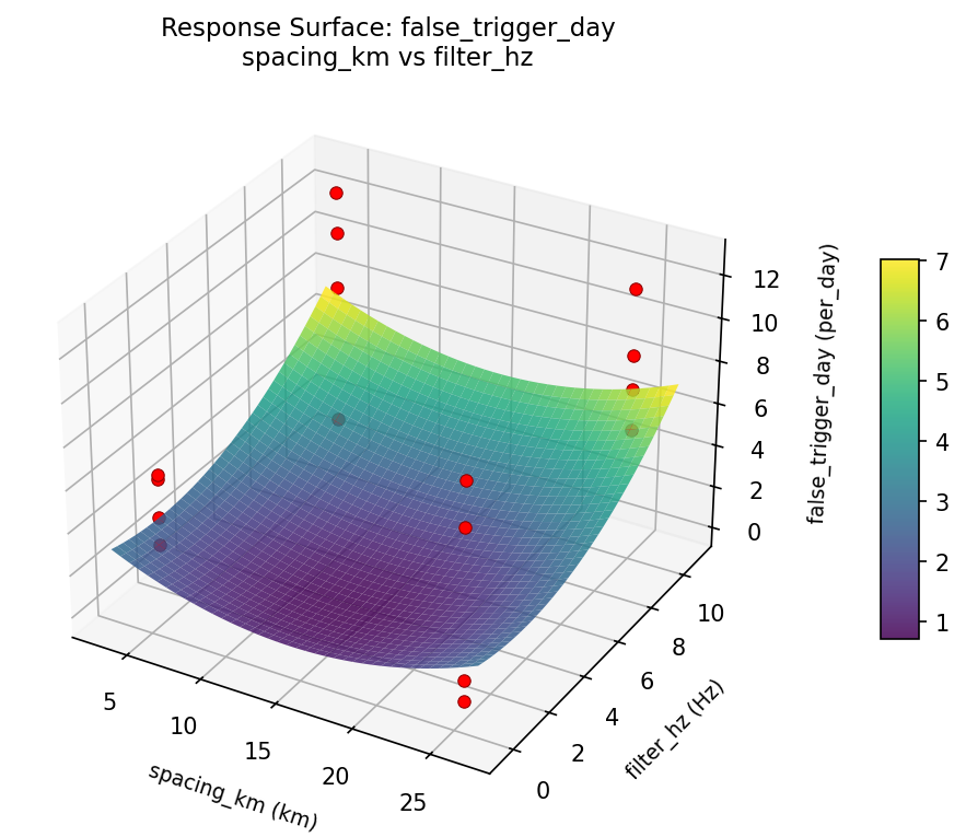
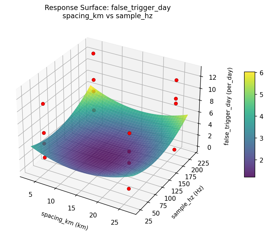
Response Surface Plots
3D surfaces fitted with quadratic RSM. Red dots are observed data points.
detection pct burial m vs filter hz
detection pct burial m vs sample hz
detection pct sample hz vs filter hz
detection pct spacing km vs burial m
detection pct spacing km vs filter hz
detection pct spacing km vs sample hz
false trigger day burial m vs filter hz
false trigger day burial m vs sample hz
false trigger day sample hz vs filter hz

false trigger day spacing km vs burial m
false trigger day spacing km vs filter hz
false trigger day spacing km vs sample hz
Multi-Objective Optimization
When responses compete, Derringer–Suich desirability finds the best compromise.
Each response is scaled to a 0–1 desirability, then combined via a weighted geometric mean.
Overall Desirability
D = 0.7819
Per-Response Desirability
| Response | Weight | Desirability | Predicted | Dir |
|---|
detection_pct |
1.5 |
|
97.00 0.8808 97.00 % |
↑ |
false_trigger_day |
1.0 |
|
4.20 0.6539 4.20 per_day |
↓ |
Recommended Settings
| Factor | Value |
|---|
spacing_km | 25 km |
burial_m | 0 m |
sample_hz | 40 Hz |
filter_hz | 10 Hz |
Source: from observed run #1
Trade-off Summary
Sacrifice = how much worse than single-objective best.
| Response | Predicted | Best Observed | Sacrifice |
|---|
false_trigger_day | 4.20 | -0.00 | +4.20 |
Top 3 Runs by Desirability
| Run | D | Factor Settings |
|---|
| #3 | 0.7413 | spacing_km=25, burial_m=0, sample_hz=40, filter_hz=0.5 |
| #4 | 0.6201 | spacing_km=5, burial_m=3, sample_hz=40, filter_hz=10 |
Model Quality
| Response | R² | Type |
|---|
false_trigger_day | 0.3639 | linear |
Full Multi-Objective Output
============================================================
MULTI-OBJECTIVE OPTIMIZATION
Method: Derringer-Suich Desirability Function
============================================================
Overall desirability: D = 0.7819
Response Weight Desirability Predicted Direction
---------------------------------------------------------------------
detection_pct 1.5 0.8808 97.00 % ↑
false_trigger_day 1.0 0.6539 4.20 per_day ↓
Recommended settings:
spacing_km = 25 km
burial_m = 0 m
sample_hz = 40 Hz
filter_hz = 10 Hz
(from observed run #1)
Trade-off summary:
detection_pct: 97.00 (best observed: 100.00, sacrifice: +3.00)
false_trigger_day: 4.20 (best observed: -0.00, sacrifice: +4.20)
Model quality:
detection_pct: R² = 0.3357 (linear)
false_trigger_day: R² = 0.3639 (linear)
Top 3 observed runs by overall desirability:
1. Run #1 (D=0.7819): spacing_km=25, burial_m=0, sample_hz=40, filter_hz=10
2. Run #3 (D=0.7413): spacing_km=25, burial_m=0, sample_hz=40, filter_hz=0.5
3. Run #4 (D=0.6201): spacing_km=5, burial_m=3, sample_hz=40, filter_hz=10
Full Analysis Output
=== Main Effects: detection_pct ===
Factor Effect Std Error % Contribution
--------------------------------------------------------------
sample_hz -11.5000 2.7180 55.4%
filter_hz 7.0000 2.7180 33.7%
burial_m 1.7500 2.7180 8.4%
spacing_km 0.5000 2.7180 2.4%
=== ANOVA Table: detection_pct ===
Source DF SS MS F p-value
-----------------------------------------------------------------------------
spacing_km 1 1.0000 1.0000 0.014 0.9117
burial_m 1 12.2500 12.2500 0.166 0.7002
sample_hz 1 529.0000 529.0000 7.188 0.0438
filter_hz 1 196.0000 196.0000 2.663 0.1636
spacing_km*burial_m 1 12.2500 12.2500 0.166 0.7002
spacing_km*sample_hz 1 196.0000 196.0000 2.663 0.1636
spacing_km*filter_hz 1 324.0000 324.0000 4.402 0.0900
burial_m*sample_hz 1 42.2500 42.2500 0.574 0.4828
burial_m*filter_hz 1 56.2500 56.2500 0.764 0.4220
sample_hz*filter_hz 1 36.0000 36.0000 0.489 0.5155
Error 5 368.0000 73.6000
Total 15 1773.0000 118.2000
=== Interaction Effects: detection_pct ===
Factor A Factor B Interaction % Contribution
------------------------------------------------------------------------
spacing_km filter_hz 9.0000 32.4%
spacing_km sample_hz 7.0000 25.2%
burial_m filter_hz 3.7500 13.5%
burial_m sample_hz 3.2500 11.7%
sample_hz filter_hz 3.0000 10.8%
spacing_km burial_m 1.7500 6.3%
=== Summary Statistics: detection_pct ===
spacing_km:
Level N Mean Std Min Max
------------------------------------------------------------
25 8 81.0000 11.3263 68.0000 100.0000
5 8 81.5000 11.1739 63.0000 97.0000
burial_m:
Level N Mean Std Min Max
------------------------------------------------------------
0 8 80.3750 11.6243 63.0000 100.0000
3 8 82.1250 10.7894 68.0000 97.0000
sample_hz:
Level N Mean Std Min Max
------------------------------------------------------------
200 8 87.0000 10.0143 68.0000 100.0000
40 8 75.5000 8.7994 63.0000 89.0000
filter_hz:
Level N Mean Std Min Max
------------------------------------------------------------
0.5 8 77.7500 12.4298 63.0000 100.0000
10 8 84.7500 8.4134 72.0000 97.0000
=== Main Effects: false_trigger_day ===
Factor Effect Std Error % Contribution
--------------------------------------------------------------
filter_hz 1.6375 0.9672 34.1%
spacing_km 1.4125 0.9672 29.4%
burial_m -1.0875 0.9672 22.7%
sample_hz 0.6625 0.9672 13.8%
=== ANOVA Table: false_trigger_day ===
Source DF SS MS F p-value
-----------------------------------------------------------------------------
spacing_km 1 7.9806 7.9806 0.555 0.4897
burial_m 1 4.7306 4.7306 0.329 0.5910
sample_hz 1 1.7556 1.7556 0.122 0.7409
filter_hz 1 10.7256 10.7256 0.746 0.4271
spacing_km*burial_m 1 1.6256 1.6256 0.113 0.7503
spacing_km*sample_hz 1 5.4056 5.4056 0.376 0.5665
spacing_km*filter_hz 1 0.0756 0.0756 0.005 0.9450
burial_m*sample_hz 1 11.3906 11.3906 0.793 0.4141
burial_m*filter_hz 1 72.6756 72.6756 5.058 0.0744
sample_hz*filter_hz 1 36.3006 36.3006 2.526 0.1728
Error 5 71.8481 14.3696
Total 15 224.5144 14.9676
=== Interaction Effects: false_trigger_day ===
Factor A Factor B Interaction % Contribution
------------------------------------------------------------------------
burial_m filter_hz 4.2625 39.1%
sample_hz filter_hz 3.0125 27.6%
burial_m sample_hz 1.6875 15.5%
spacing_km sample_hz -1.1625 10.7%
spacing_km burial_m 0.6375 5.8%
spacing_km filter_hz -0.1375 1.3%
=== Summary Statistics: false_trigger_day ===
spacing_km:
Level N Mean Std Min Max
------------------------------------------------------------
25 8 5.8625 4.3270 -0.0000 10.8000
5 8 7.2750 3.4944 2.9000 12.7000
burial_m:
Level N Mean Std Min Max
------------------------------------------------------------
0 8 7.1125 3.4286 1.8000 11.9000
3 8 6.0250 4.4319 -0.0000 12.7000
sample_hz:
Level N Mean Std Min Max
------------------------------------------------------------
200 8 6.2375 3.7210 1.0000 11.9000
40 8 6.9000 4.2399 -0.0000 12.7000
filter_hz:
Level N Mean Std Min Max
------------------------------------------------------------
0.5 8 5.7500 4.3105 -0.0000 11.9000
10 8 7.3875 3.4585 1.8000 12.7000
Optimization Recommendations
=== Optimization: detection_pct ===
Direction: maximize
Best observed run: #4
spacing_km = 5
burial_m = 3
sample_hz = 200
filter_hz = 0.5
Value: 100.0
RSM Model (linear, R² = 0.1514, Adj R² = -0.1571):
Coefficients:
intercept +81.2500
spacing_km -1.5000
burial_m -0.6250
sample_hz +3.6250
filter_hz -1.0000
RSM Model (quadratic, R² = 0.2941, Adj R² = -9.5880):
Coefficients:
intercept +16.2500
spacing_km -1.5000
burial_m -0.6250
sample_hz +3.6250
filter_hz -1.0000
spacing_km*burial_m -1.1250
spacing_km*sample_hz -1.3750
spacing_km*filter_hz -3.0000
burial_m*sample_hz +0.0000
burial_m*filter_hz -0.3750
sample_hz*filter_hz +1.8750
spacing_km^2 +16.2500
burial_m^2 +16.2500
sample_hz^2 +16.2500
filter_hz^2 +16.2500
Curvature analysis:
spacing_km coef=+16.2500 convex (has a minimum)
burial_m coef=+16.2500 convex (has a minimum)
sample_hz coef=+16.2500 convex (has a minimum)
filter_hz coef=+16.2500 convex (has a minimum)
Notable interactions:
spacing_km*filter_hz coef=-3.0000 (antagonistic)
sample_hz*filter_hz coef=+1.8750 (synergistic)
spacing_km*sample_hz coef=-1.3750 (antagonistic)
spacing_km*burial_m coef=-1.1250 (antagonistic)
burial_m*filter_hz coef=-0.3750 (antagonistic)
Predicted optimum (from linear model, at observed points):
spacing_km = 5
burial_m = 0
sample_hz = 200
filter_hz = 0.5
Predicted value: 88.0000
Surface optimum (via L-BFGS-B, linear model):
spacing_km = 5
burial_m = 0
sample_hz = 200
filter_hz = 0.5
Predicted value: 88.0000
Model quality: Weak fit — consider adding center points or using a different design.
Factor importance:
1. sample_hz (effect: -7.2, contribution: 53.7%)
2. spacing_km (effect: 3.0, contribution: 22.2%)
3. filter_hz (effect: -2.0, contribution: 14.8%)
4. burial_m (effect: -1.2, contribution: 9.3%)
=== Optimization: false_trigger_day ===
Direction: minimize
Best observed run: #11
spacing_km = 25
burial_m = 3
sample_hz = 200
filter_hz = 10
Value: -0.0
RSM Model (linear, R² = 0.1293, Adj R² = -0.1873):
Coefficients:
intercept +6.5688
spacing_km -1.0313
burial_m -0.2813
sample_hz -0.8187
filter_hz -0.0437
RSM Model (quadratic, R² = 0.6693, Adj R² = -3.9602):
Coefficients:
intercept +1.3137
spacing_km -1.0312
burial_m -0.2813
sample_hz -0.8187
filter_hz -0.0438
spacing_km*burial_m -0.5813
spacing_km*sample_hz +0.0313
spacing_km*filter_hz -1.1688
burial_m*sample_hz +0.0563
burial_m*filter_hz +0.2813
sample_hz*filter_hz -2.4063
spacing_km^2 +1.3138
burial_m^2 +1.3138
sample_hz^2 +1.3137
filter_hz^2 +1.3138
Curvature analysis:
spacing_km coef=+1.3138 convex (has a minimum)
burial_m coef=+1.3138 convex (has a minimum)
filter_hz coef=+1.3138 convex (has a minimum)
sample_hz coef=+1.3137 convex (has a minimum)
Notable interactions:
sample_hz*filter_hz coef=-2.4063 (antagonistic)
spacing_km*filter_hz coef=-1.1688 (antagonistic)
spacing_km*burial_m coef=-0.5813 (antagonistic)
Predicted optimum (from linear model, at observed points):
spacing_km = 5
burial_m = 0
sample_hz = 40
filter_hz = 0.5
Predicted value: 8.7438
Surface optimum (via L-BFGS-B, linear model):
spacing_km = 25
burial_m = 3
sample_hz = 200
filter_hz = 10
Predicted value: 4.3938
Model quality: Weak fit — consider adding center points or using a different design.
Factor importance:
1. spacing_km (effect: 2.1, contribution: 47.4%)
2. sample_hz (effect: 1.6, contribution: 37.6%)
3. burial_m (effect: -0.6, contribution: 12.9%)
4. filter_hz (effect: -0.1, contribution: 2.0%)