Summary
This experiment investigates mineral flotation separation. Central composite design to maximize mineral recovery and grade by tuning collector dosage, frother concentration, and pulp pH.
The design varies 3 factors: collector g t (g/t), ranging from 20 to 80, frother g t (g/t), ranging from 10 to 40, and pulp ph (pH), ranging from 7 to 11. The goal is to optimize 2 responses: recovery pct (%) (maximize) and grade pct (%Cu) (maximize). Fixed conditions held constant across all runs include mineral = chalcopyrite, grind size = 75um.
A Central Composite Design (CCD) was selected to fit a full quadratic response surface model, including curvature and interaction effects. With 3 factors this produces 22 runs including center points and axial (star) points that extend beyond the factorial range.
Quadratic response surface models were fitted to capture potential curvature and factor interactions. The RSM contour plots below visualize how pairs of factors jointly affect each response.
Key Findings
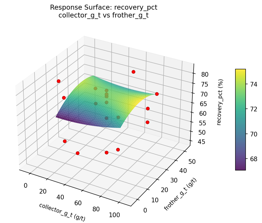
For recovery pct, the most influential factors were collector g t (35.0%), pulp ph (34.0%), frother g t (31.0%). The best observed value was 82.0 (at collector g t = 50, frother g t = 52.3861, pulp ph = 9).
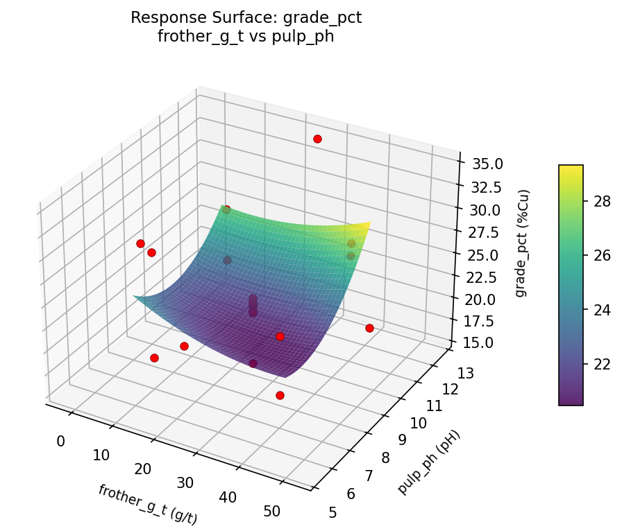
For grade pct, the most influential factors were frother g t (57.4%), pulp ph (24.6%), collector g t (18.0%). The best observed value was 34.6 (at collector g t = 50, frother g t = 25, pulp ph = 9).
Recommended Next Steps
- Run confirmation experiments at the predicted optimal settings to validate the model.
- Consider whether any fixed factors should be varied in a future study.
Experimental Setup
Factors
| Factor | Low | High | Unit |
|---|
collector_g_t | 20 | 80 | g/t |
frother_g_t | 10 | 40 | g/t |
pulp_ph | 7 | 11 | pH |
Fixed: mineral = chalcopyrite, grind_size = 75um
Responses
| Response | Direction | Unit |
|---|
recovery_pct | ↑ maximize | % |
grade_pct | ↑ maximize | %Cu |
Configuration
{
"metadata": {
"name": "Mineral Flotation Separation",
"description": "Central composite design to maximize mineral recovery and grade by tuning collector dosage, frother concentration, and pulp pH"
},
"factors": [
{
"name": "collector_g_t",
"levels": [
"20",
"80"
],
"type": "continuous",
"unit": "g/t"
},
{
"name": "frother_g_t",
"levels": [
"10",
"40"
],
"type": "continuous",
"unit": "g/t"
},
{
"name": "pulp_ph",
"levels": [
"7",
"11"
],
"type": "continuous",
"unit": "pH"
}
],
"fixed_factors": {
"mineral": "chalcopyrite",
"grind_size": "75um"
},
"responses": [
{
"name": "recovery_pct",
"optimize": "maximize",
"unit": "%"
},
{
"name": "grade_pct",
"optimize": "maximize",
"unit": "%Cu"
}
],
"settings": {
"operation": "central_composite",
"test_script": "use_cases/234_mineral_flotation/sim.sh"
}
}
Experimental Matrix
The Central Composite Design produces 22 runs. Each row is one experiment with specific factor settings.
| Run | collector_g_t | frother_g_t | pulp_ph |
|---|
| 1 | 50 | 25 | 9 |
| 2 | 80 | 10 | 11 |
| 3 | 20 | 40 | 7 |
| 4 | 50 | 52.3861 | 9 |
| 5 | 50 | 25 | 9 |
| 6 | -4.77226 | 25 | 9 |
| 7 | 50 | 25 | 5.34852 |
| 8 | 50 | 25 | 9 |
| 9 | 80 | 40 | 7 |
| 10 | 104.772 | 25 | 9 |
| 11 | 50 | 25 | 9 |
| 12 | 50 | -2.38613 | 9 |
| 13 | 50 | 25 | 9 |
| 14 | 20 | 10 | 11 |
| 15 | 50 | 25 | 9 |
| 16 | 80 | 10 | 7 |
| 17 | 50 | 25 | 12.6515 |
| 18 | 80 | 40 | 11 |
| 19 | 50 | 25 | 9 |
| 20 | 20 | 10 | 7 |
| 21 | 20 | 40 | 11 |
| 22 | 50 | 25 | 9 |
Step-by-Step Workflow
1
Preview the design
$ doe info --config use_cases/234_mineral_flotation/config.json
2
Generate the runner script
$ doe generate --config use_cases/234_mineral_flotation/config.json \
--output use_cases/234_mineral_flotation/results/run.sh --seed 42
3
Execute the experiments
$ bash use_cases/234_mineral_flotation/results/run.sh
4
Analyze results
$ doe analyze --config use_cases/234_mineral_flotation/config.json
5
Get optimization recommendations
$ doe optimize --config use_cases/234_mineral_flotation/config.json
6
Multi-objective optimization
With 2 competing responses, use --multi to find the best compromise via Derringer–Suich desirability.
$ doe optimize --config use_cases/234_mineral_flotation/config.json --multi
7
Generate the HTML report
$ doe report --config use_cases/234_mineral_flotation/config.json \
--output use_cases/234_mineral_flotation/results/report.html
Features Exercised
| Feature | Value |
|---|
| Design type | central_composite |
| Factor types | continuous (all 3) |
| Arg style | double-dash |
| Responses | 2 (recovery_pct ↑, grade_pct ↑) |
| Total runs | 22 |
Analysis Results
Generated from actual experiment runs using the DOE Helper Tool.
Response: recovery_pct
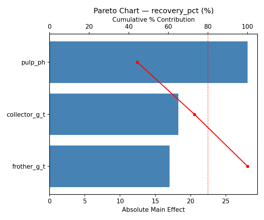
Top factors: collector_g_t (35.0%), pulp_ph (34.0%), frother_g_t (31.0%).
ANOVA
| Source | DF | SS | MS | F | p-value |
|---|
| Source | DF | SS | MS | F | p-value |
| collector_g_t | 4 | 426.0379 | 106.5095 | 1.487 | 0.2846 |
| frother_g_t | 4 | 243.0379 | 60.7595 | 0.848 | 0.5291 |
| pulp_ph | 4 | 228.0379 | 57.0095 | 0.796 | 0.5569 |
| Lack | of | Fit | 2 | 458.8409 | 229.4205 |
| Pure | Error | 7 | 501.5000 | | |
| Error | 9 | 960.3409 | 71.6429 | | |
| Total | 21 | 1857.4545 | 88.4502 | | |
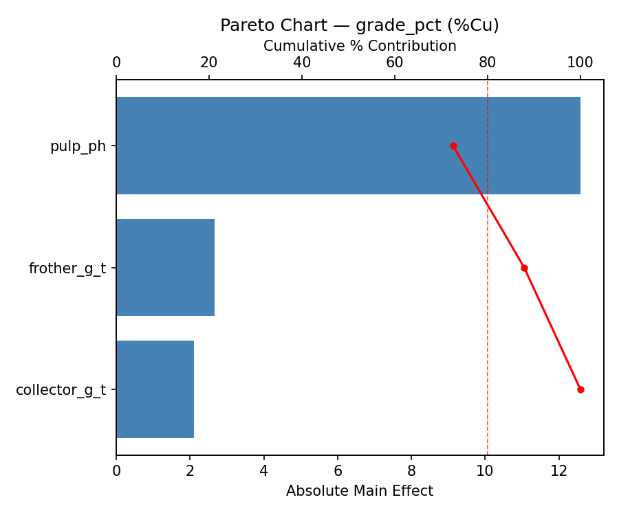
Pareto Chart
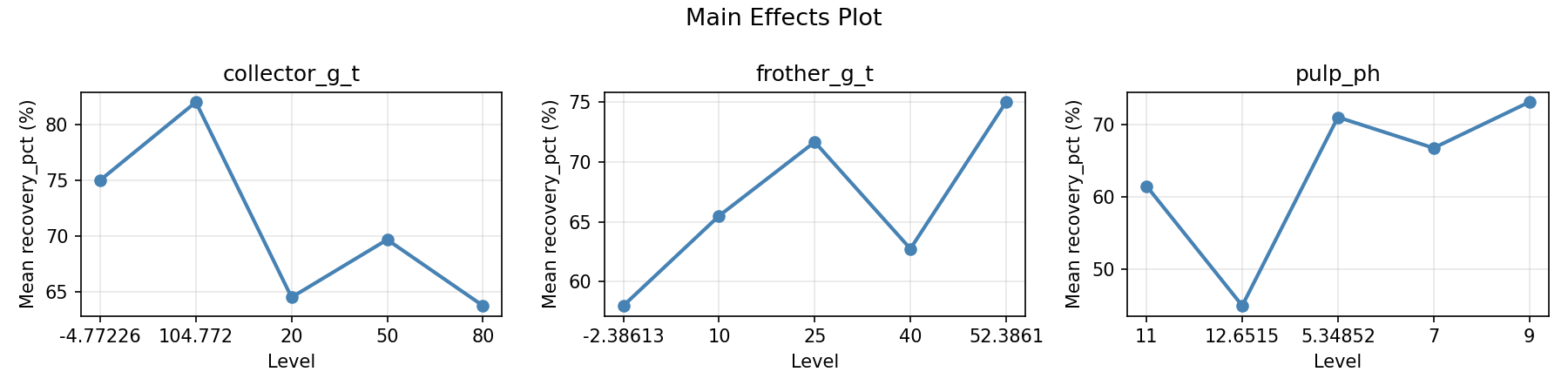
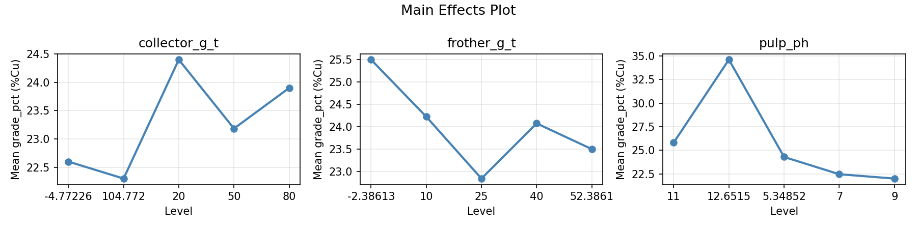
Main Effects Plot
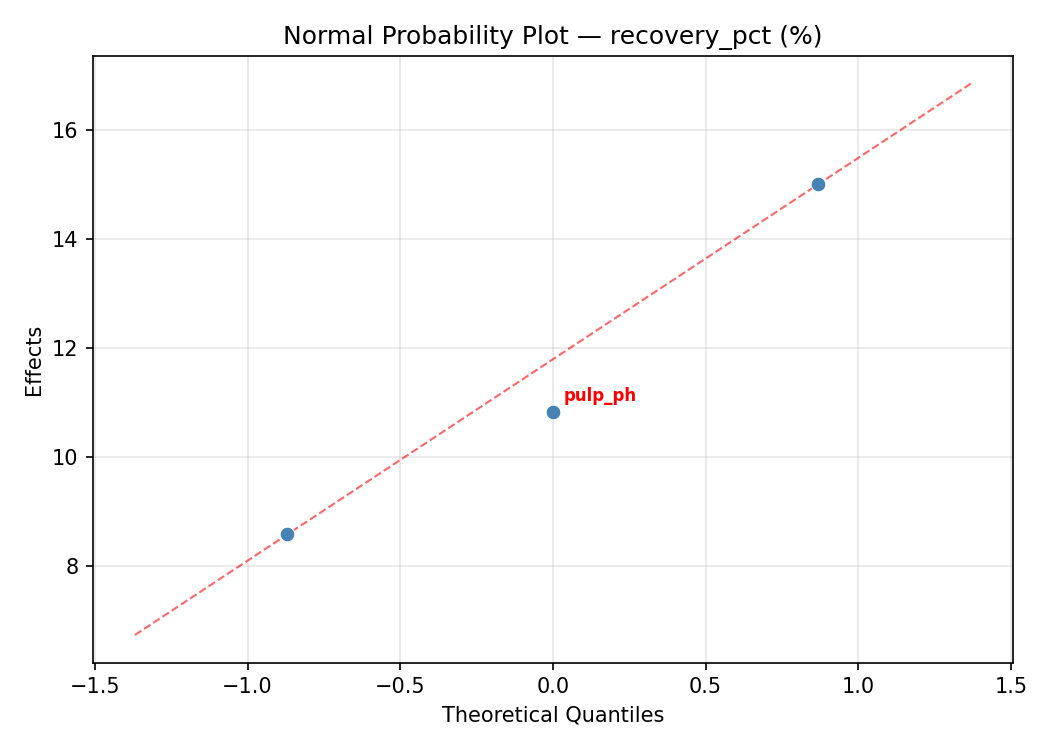
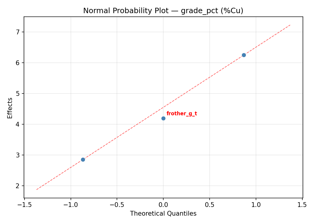
Normal Probability Plot of Effects
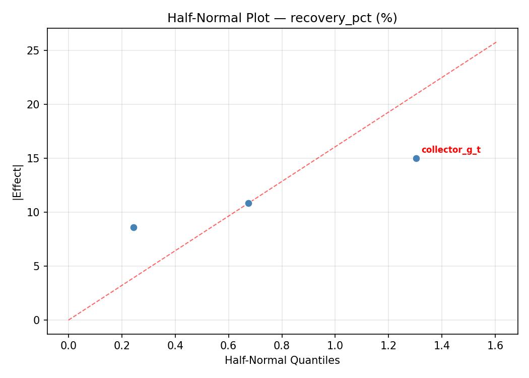
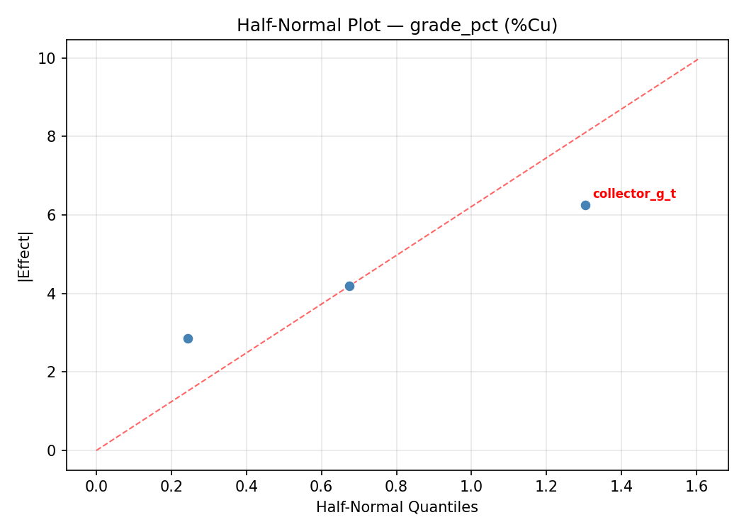
Half-Normal Plot of Effects
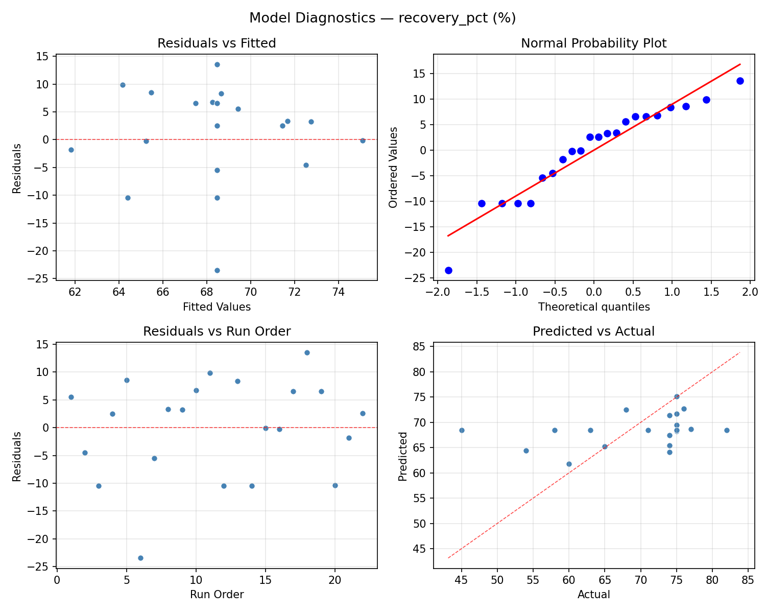
Model Diagnostics
Response: grade_pct
Top factors: frother_g_t (57.4%), pulp_ph (24.6%), collector_g_t (18.0%).
ANOVA
| Source | DF | SS | MS | F | p-value |
|---|
| Source | DF | SS | MS | F | p-value |
| collector_g_t | 4 | 9.8036 | 2.4509 | 0.224 | 0.9185 |
| frother_g_t | 4 | 67.2111 | 16.8028 | 1.533 | 0.2725 |
| pulp_ph | 4 | 54.2777 | 13.5694 | 1.238 | 0.3612 |
| Lack | of | Fit | 2 | 140.9954 | 70.4977 |
| Pure | Error | 7 | 76.7200 | | |
| Error | 9 | 217.7154 | 10.9600 | | |
| Total | 21 | 349.0077 | 16.6194 | | |
Pareto Chart
Main Effects Plot
Normal Probability Plot of Effects
Half-Normal Plot of Effects
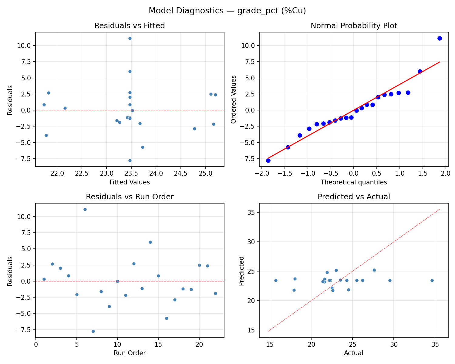
Model Diagnostics
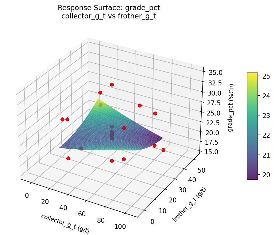
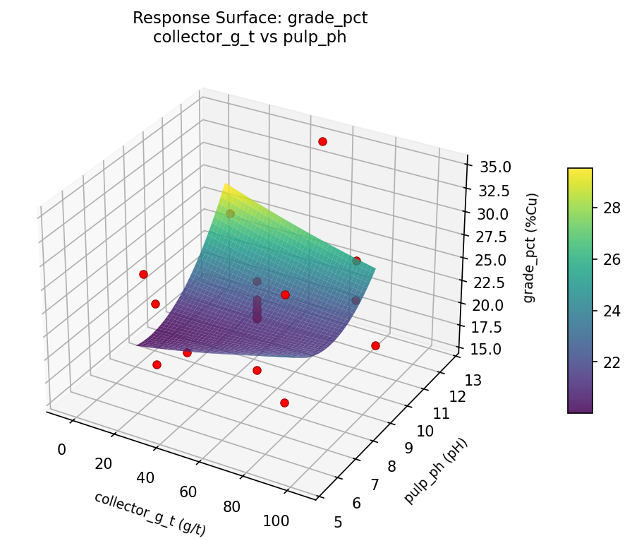
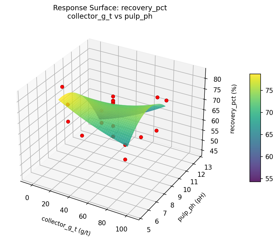
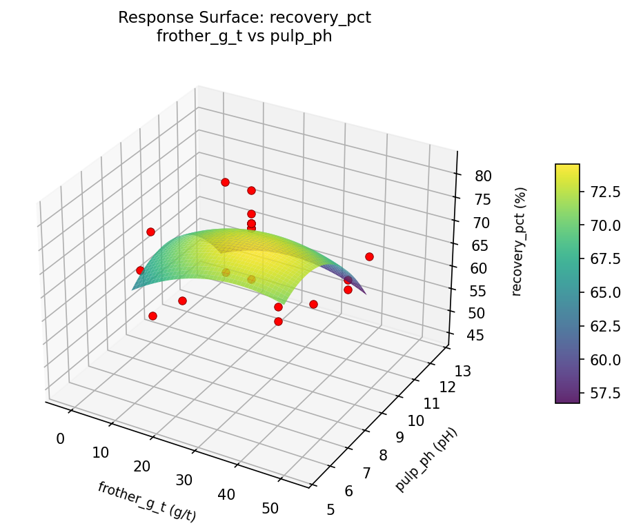
Response Surface Plots
3D surfaces fitted with quadratic RSM. Red dots are observed data points.
grade pct collector g t vs frother g t
grade pct collector g t vs pulp ph
grade pct frother g t vs pulp ph
recovery pct collector g t vs frother g t
recovery pct collector g t vs pulp ph
recovery pct frother g t vs pulp ph
Multi-Objective Optimization
When responses compete, Derringer–Suich desirability finds the best compromise.
Each response is scaled to a 0–1 desirability, then combined via a weighted geometric mean.
Overall Desirability
D = 0.5451
Per-Response Desirability
| Response | Weight | Desirability | Predicted | Dir |
|---|
recovery_pct |
1.0 |
|
67.93 0.6089 67.93 % |
↑ |
grade_pct |
1.5 |
|
25.28 0.5063 25.28 %Cu |
↑ |
Recommended Settings
| Factor | Value |
|---|
collector_g_t | 80 g/t |
frother_g_t | 10 g/t |
pulp_ph | 11 pH |
Source: from RSM model prediction
Trade-off Summary
Sacrifice = how much worse than single-objective best.
| Response | Predicted | Best Observed | Sacrifice |
|---|
grade_pct | 25.28 | 34.60 | +9.32 |
Top 3 Runs by Desirability
| Run | D | Factor Settings |
|---|
| #10 | 0.5392 | collector_g_t=50, frother_g_t=25, pulp_ph=12.6515 |
| #4 | 0.5386 | collector_g_t=50, frother_g_t=25, pulp_ph=9 |
Model Quality
| Response | R² | Type |
|---|
grade_pct | 0.0800 | linear |
Full Multi-Objective Output
============================================================
MULTI-OBJECTIVE OPTIMIZATION
Method: Derringer-Suich Desirability Function
============================================================
Overall desirability: D = 0.5451
Response Weight Desirability Predicted Direction
---------------------------------------------------------------------
recovery_pct 1.0 0.6089 67.93 % ↑
grade_pct 1.5 0.5063 25.28 %Cu ↑
Recommended settings:
collector_g_t = 80 g/t
frother_g_t = 10 g/t
pulp_ph = 11 pH
(from RSM model prediction)
Trade-off summary:
recovery_pct: 67.93 (best observed: 82.00, sacrifice: +14.07)
grade_pct: 25.28 (best observed: 34.60, sacrifice: +9.32)
Model quality:
recovery_pct: R² = 0.0753 (linear)
grade_pct: R² = 0.0800 (linear)
Top 3 observed runs by overall desirability:
1. Run #14 (D=0.5437): collector_g_t=50, frother_g_t=-2.38613, pulp_ph=9
2. Run #10 (D=0.5392): collector_g_t=50, frother_g_t=25, pulp_ph=12.6515
3. Run #4 (D=0.5386): collector_g_t=50, frother_g_t=25, pulp_ph=9
Full Analysis Output
=== Main Effects: recovery_pct ===
Factor Effect Std Error % Contribution
--------------------------------------------------------------
collector_g_t 17.5000 2.0051 35.0%
pulp_ph 17.0000 2.0051 34.0%
frother_g_t 15.5000 2.0051 31.0%
=== ANOVA Table: recovery_pct ===
Source DF SS MS F p-value
-----------------------------------------------------------------------------
collector_g_t 4 426.0379 106.5095 1.487 0.2846
frother_g_t 4 243.0379 60.7595 0.848 0.5291
pulp_ph 4 228.0379 57.0095 0.796 0.5569
Lack of Fit 2 458.8409 229.4205 3.202 0.1029
Pure Error 7 501.5000 71.6429
Error 9 960.3409 71.6429
Total 21 1857.4545 88.4502
=== Summary Statistics: recovery_pct ===
collector_g_t:
Level N Mean Std Min Max
------------------------------------------------------------
-4.77226 1 58.0000 0.0000 58.0000 58.0000
104.772 1 75.0000 0.0000 75.0000 75.0000
20 4 75.5000 4.6547 71.0000 82.0000
50 12 67.8333 8.4405 54.0000 77.0000
80 4 64.2500 13.9374 45.0000 75.0000
frother_g_t:
Level N Mean Std Min Max
------------------------------------------------------------
-2.38613 1 58.0000 0.0000 58.0000 58.0000
10 4 73.5000 1.7321 71.0000 75.0000
25 12 68.6667 8.6269 54.0000 77.0000
40 4 66.2500 16.1941 45.0000 82.0000
52.3861 1 65.0000 0.0000 65.0000 65.0000
pulp_ph:
Level N Mean Std Min Max
------------------------------------------------------------
11 4 72.5000 7.8528 63.0000 82.0000
12.6515 1 58.0000 0.0000 58.0000 58.0000
5.34852 1 75.0000 0.0000 75.0000 75.0000
7 4 67.2500 14.8408 45.0000 75.0000
9 12 67.8333 8.4405 54.0000 77.0000
=== Main Effects: grade_pct ===
Factor Effect Std Error % Contribution
--------------------------------------------------------------
frother_g_t 11.5000 0.8692 57.4%
pulp_ph 4.9250 0.8692 24.6%
collector_g_t 3.6000 0.8692 18.0%
=== ANOVA Table: grade_pct ===
Source DF SS MS F p-value
-----------------------------------------------------------------------------
collector_g_t 4 9.8036 2.4509 0.224 0.9185
frother_g_t 4 67.2111 16.8028 1.533 0.2725
pulp_ph 4 54.2777 13.5694 1.238 0.3612
Lack of Fit 2 140.9954 70.4977 6.432 0.0260
Pure Error 7 76.7200 10.9600
Error 9 217.7154 10.9600
Total 21 349.0077 16.6194
=== Summary Statistics: grade_pct ===
collector_g_t:
Level N Mean Std Min Max
------------------------------------------------------------
-4.77226 1 26.2000 0.0000 26.2000 26.2000
104.772 1 22.6000 0.0000 22.6000 22.6000
20 4 23.0250 0.8995 22.3000 24.3000
50 12 23.3333 3.6879 17.9000 29.5000
80 4 23.8500 7.8987 15.7000 34.6000
frother_g_t:
Level N Mean Std Min Max
------------------------------------------------------------
-2.38613 1 29.5000 0.0000 29.5000 29.5000
10 4 23.1000 1.1343 21.6000 24.3000
25 12 23.4417 2.8881 17.9000 27.6000
40 4 23.7750 7.8780 15.7000 34.6000
52.3861 1 18.0000 0.0000 18.0000 18.0000
pulp_ph:
Level N Mean Std Min Max
------------------------------------------------------------
11 4 20.9750 3.6981 15.7000 24.3000
12.6515 1 25.5000 0.0000 25.5000 25.5000
5.34852 1 22.2000 0.0000 22.2000 22.2000
7 4 25.9000 5.8144 22.5000 34.6000
9 12 23.4250 3.7207 17.9000 29.5000
Optimization Recommendations
=== Optimization: recovery_pct ===
Direction: maximize
Best observed run: #18
collector_g_t = 50
frother_g_t = 52.3861
pulp_ph = 9
Value: 82.0
RSM Model (linear, R² = 0.2288, Adj R² = 0.1003):
Coefficients:
intercept +68.4545
collector_g_t +2.8724
frother_g_t +3.4173
pulp_ph -3.0088
RSM Model (quadratic, R² = 0.3913, Adj R² = -0.0652):
Coefficients:
intercept +67.5203
collector_g_t +2.8724
frother_g_t +3.4173
pulp_ph -3.0088
collector_g_t*frother_g_t +0.1250
collector_g_t*pulp_ph +3.8750
frother_g_t*pulp_ph +0.1250
collector_g_t^2 +2.3171
frother_g_t^2 +0.6671
pulp_ph^2 -1.5829
Curvature analysis:
collector_g_t coef=+2.3171 convex (has a minimum)
pulp_ph coef=-1.5829 concave (has a maximum)
frother_g_t coef=+0.6671 convex (has a minimum)
Notable interactions:
collector_g_t*pulp_ph coef=+3.8750 (synergistic)
Predicted optimum (from linear model, at observed points):
collector_g_t = 80
frother_g_t = 40
pulp_ph = 7
Predicted value: 77.7531
Surface optimum (via L-BFGS-B, linear model):
collector_g_t = 80
frother_g_t = 40
pulp_ph = 7
Predicted value: 77.7531
Model quality: Weak fit — consider adding center points or using a different design.
Factor importance:
1. frother_g_t (effect: 28.0, contribution: 51.4%)
2. pulp_ph (effect: 16.8, contribution: 30.7%)
3. collector_g_t (effect: 9.8, contribution: 17.9%)
=== Optimization: grade_pct ===
Direction: maximize
Best observed run: #6
collector_g_t = 50
frother_g_t = 25
pulp_ph = 9
Value: 34.6
RSM Model (linear, R² = 0.2679, Adj R² = 0.1458):
Coefficients:
intercept +23.4682
collector_g_t -1.5944
frother_g_t -0.4348
pulp_ph +1.9086
RSM Model (quadratic, R² = 0.4358, Adj R² = 0.0127):
Coefficients:
intercept +24.4379
collector_g_t -1.5944
frother_g_t -0.4348
pulp_ph +1.9086
collector_g_t*frother_g_t -0.1875
collector_g_t*pulp_ph -1.6375
frother_g_t*pulp_ph +0.5375
collector_g_t^2 -0.8199
frother_g_t^2 +0.3351
pulp_ph^2 -0.9699
Curvature analysis:
pulp_ph coef=-0.9699 concave (has a maximum)
collector_g_t coef=-0.8199 concave (has a maximum)
frother_g_t coef=+0.3351 convex (has a minimum)
Notable interactions:
collector_g_t*pulp_ph coef=-1.6375 (antagonistic)
frother_g_t*pulp_ph coef=+0.5375 (synergistic)
Predicted optimum (from linear model, at observed points):
collector_g_t = 20
frother_g_t = 10
pulp_ph = 11
Predicted value: 27.4059
Surface optimum (via L-BFGS-B, linear model):
collector_g_t = 20
frother_g_t = 10
pulp_ph = 11
Predicted value: 27.4059
Model quality: Weak fit — consider adding center points or using a different design.
Factor importance:
1. pulp_ph (effect: 9.8, contribution: 44.2%)
2. collector_g_t (effect: 7.1, contribution: 31.8%)
3. frother_g_t (effect: 5.3, contribution: 23.9%)