Summary
This experiment investigates sauerkraut fermentation. Full factorial of salt concentration, cabbage shred width, temperature, and pressing weight to maximize tang and crunch.
The design varies 4 factors: salt pct (%), ranging from 2 to 4, shred mm (mm), ranging from 2 to 6, temp c (C), ranging from 15 to 25, and weight kg (kg), ranging from 1 to 5. The goal is to optimize 2 responses: tang score (pts) (maximize) and crunch score (pts) (maximize). Fixed conditions held constant across all runs include cabbage = green, vessel = crock.
A full factorial design was used to explore all 16 possible combinations of the 4 factors at two levels. This guarantees that every main effect and interaction can be estimated independently, at the cost of a larger experiment (16 runs).
Quadratic response surface models were fitted to capture potential curvature and factor interactions. The RSM contour plots below visualize how pairs of factors jointly affect each response.
Key Findings
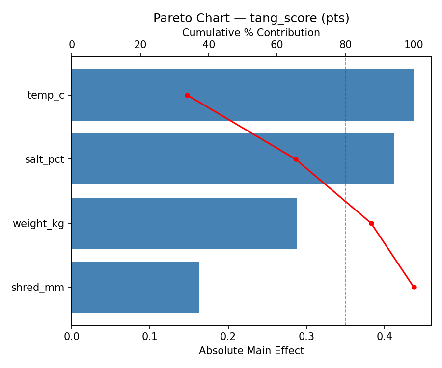
For tang score, the most influential factors were salt pct (63.8%), shred mm (19.0%), weight kg (12.1%). The best observed value was 7.0 (at salt pct = 2, shred mm = 2, temp c = 25).
For crunch score, the most influential factors were temp c (42.4%), shred mm (40.9%), weight kg (10.6%). The best observed value was 8.5 (at salt pct = 2, shred mm = 2, temp c = 25).
Recommended Next Steps
- Consider whether any fixed factors should be varied in a future study.
Experimental Setup
Factors
| Factor | Low | High | Unit |
|---|
salt_pct | 2 | 4 | % |
shred_mm | 2 | 6 | mm |
temp_c | 15 | 25 | C |
weight_kg | 1 | 5 | kg |
Fixed: cabbage = green, vessel = crock
Responses
| Response | Direction | Unit |
|---|
tang_score | ↑ maximize | pts |
crunch_score | ↑ maximize | pts |
Configuration
{
"metadata": {
"name": "Sauerkraut Fermentation",
"description": "Full factorial of salt concentration, cabbage shred width, temperature, and pressing weight to maximize tang and crunch"
},
"factors": [
{
"name": "salt_pct",
"levels": [
"2",
"4"
],
"type": "continuous",
"unit": "%"
},
{
"name": "shred_mm",
"levels": [
"2",
"6"
],
"type": "continuous",
"unit": "mm"
},
{
"name": "temp_c",
"levels": [
"15",
"25"
],
"type": "continuous",
"unit": "C"
},
{
"name": "weight_kg",
"levels": [
"1",
"5"
],
"type": "continuous",
"unit": "kg"
}
],
"fixed_factors": {
"cabbage": "green",
"vessel": "crock"
},
"responses": [
{
"name": "tang_score",
"optimize": "maximize",
"unit": "pts"
},
{
"name": "crunch_score",
"optimize": "maximize",
"unit": "pts"
}
],
"settings": {
"operation": "full_factorial",
"test_script": "use_cases/242_sauerkraut_ferment/sim.sh"
}
}
Experimental Matrix
The Full Factorial Design produces 16 runs. Each row is one experiment with specific factor settings.
| Run | salt_pct | shred_mm | temp_c | weight_kg |
|---|
| 1 | 2 | 6 | 25 | 5 |
| 2 | 4 | 2 | 15 | 5 |
| 3 | 2 | 6 | 15 | 5 |
| 4 | 2 | 6 | 25 | 1 |
| 5 | 4 | 6 | 25 | 1 |
| 6 | 4 | 2 | 25 | 1 |
| 7 | 4 | 6 | 15 | 1 |
| 8 | 4 | 2 | 15 | 1 |
| 9 | 2 | 2 | 15 | 5 |
| 10 | 2 | 2 | 25 | 1 |
| 11 | 4 | 6 | 15 | 5 |
| 12 | 4 | 6 | 25 | 5 |
| 13 | 2 | 6 | 15 | 1 |
| 14 | 4 | 2 | 25 | 5 |
| 15 | 2 | 2 | 15 | 1 |
| 16 | 2 | 2 | 25 | 5 |
Step-by-Step Workflow
1
Preview the design
$ doe info --config use_cases/242_sauerkraut_ferment/config.json
2
Generate the runner script
$ doe generate --config use_cases/242_sauerkraut_ferment/config.json \
--output use_cases/242_sauerkraut_ferment/results/run.sh --seed 42
3
Execute the experiments
$ bash use_cases/242_sauerkraut_ferment/results/run.sh
4
Analyze results
$ doe analyze --config use_cases/242_sauerkraut_ferment/config.json
5
Get optimization recommendations
$ doe optimize --config use_cases/242_sauerkraut_ferment/config.json
6
Multi-objective optimization
With 2 competing responses, use --multi to find the best compromise via Derringer–Suich desirability.
$ doe optimize --config use_cases/242_sauerkraut_ferment/config.json --multi
7
Generate the HTML report
$ doe report --config use_cases/242_sauerkraut_ferment/config.json \
--output use_cases/242_sauerkraut_ferment/results/report.html
Features Exercised
| Feature | Value |
|---|
| Design type | full_factorial |
| Factor types | continuous (all 4) |
| Arg style | double-dash |
| Responses | 2 (tang_score ↑, crunch_score ↑) |
| Total runs | 16 |
Analysis Results
Generated from actual experiment runs using the DOE Helper Tool.
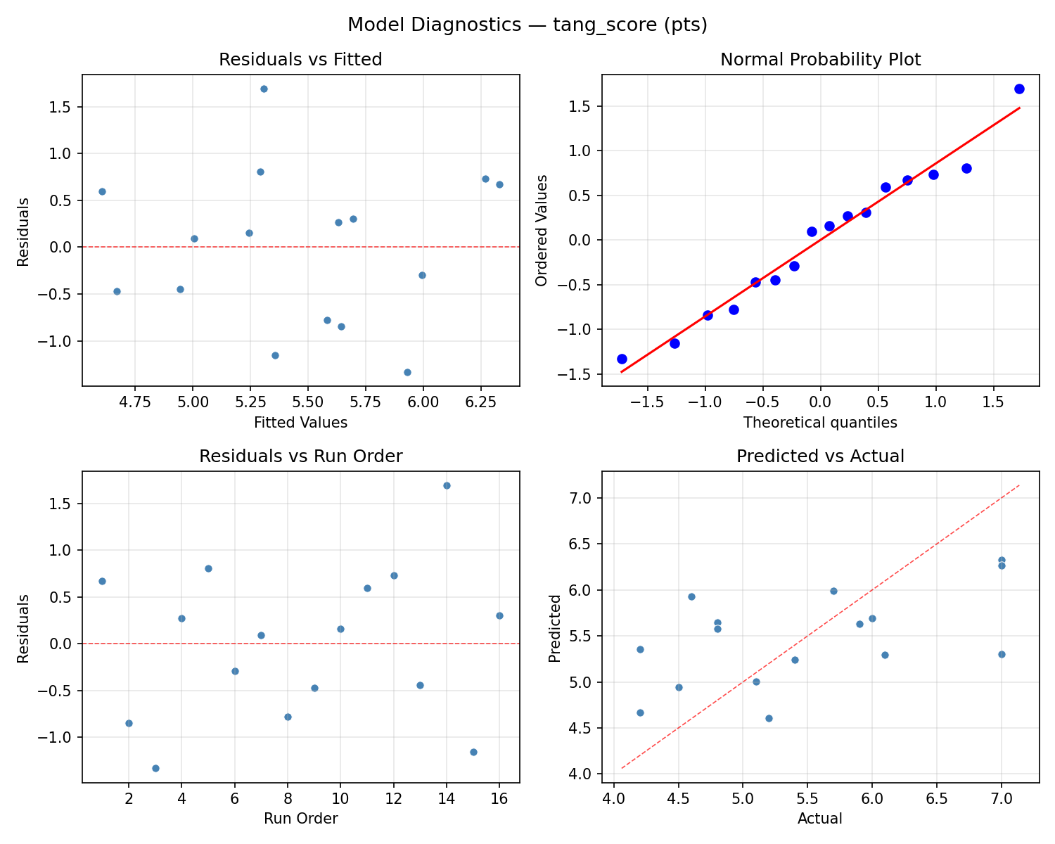
Response: tang_score
Top factors: salt_pct (63.8%), shred_mm (19.0%), weight_kg (12.1%).
ANOVA
| Source | DF | SS | MS | F | p-value |
|---|
| Source | DF | SS | MS | F | p-value |
| salt_pct | 1 | 0.8556 | 0.8556 | 1.125 | 0.3374 |
| shred_mm | 1 | 0.0756 | 0.0756 | 0.099 | 0.7653 |
| temp_c | 1 | 0.0056 | 0.0056 | 0.007 | 0.9348 |
| weight_kg | 1 | 0.0306 | 0.0306 | 0.040 | 0.8489 |
| salt_pct*shred_mm | 1 | 0.6006 | 0.6006 | 0.790 | 0.4149 |
| salt_pct*temp_c | 1 | 1.3806 | 1.3806 | 1.815 | 0.2357 |
| salt_pct*weight_kg | 1 | 0.1056 | 0.1056 | 0.139 | 0.7247 |
| shred_mm*temp_c | 1 | 5.1756 | 5.1756 | 6.804 | 0.0478 |
| shred_mm*weight_kg | 1 | 0.0506 | 0.0506 | 0.067 | 0.8067 |
| temp_c*weight_kg | 1 | 1.8906 | 1.8906 | 2.486 | 0.1757 |
| Error | 5 | 3.8031 | 0.7606 | | |
| Total | 15 | 13.9744 | 0.9316 | | |
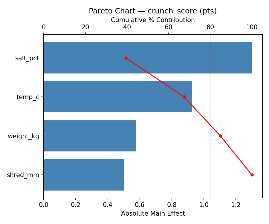
Pareto Chart
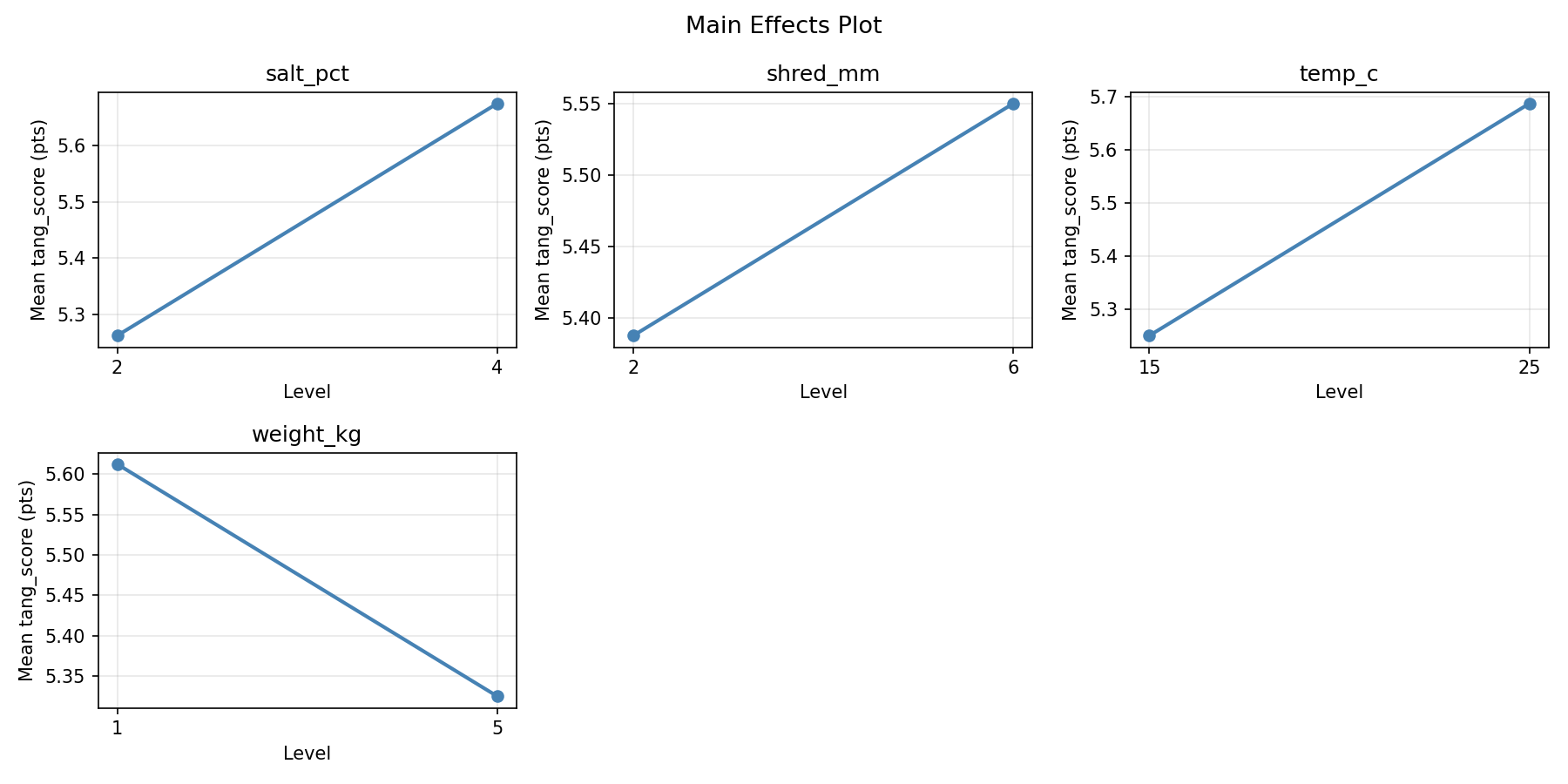
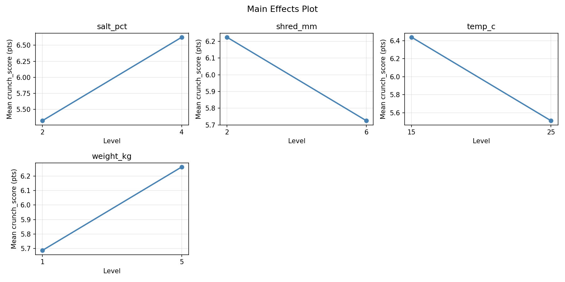
Main Effects Plot
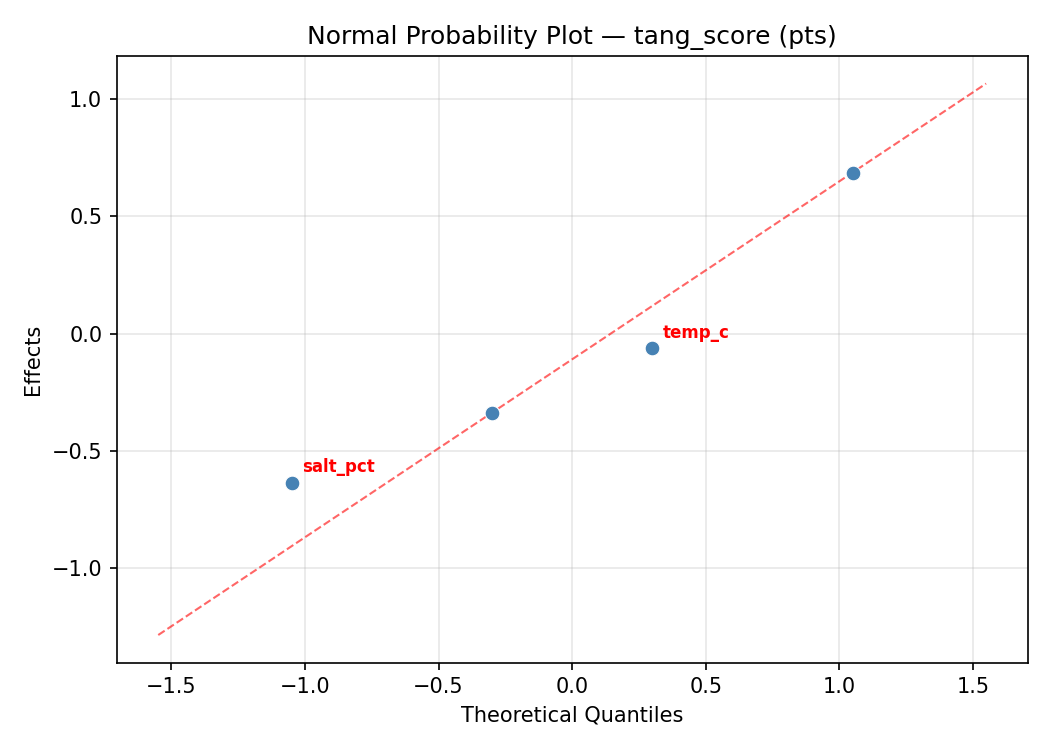
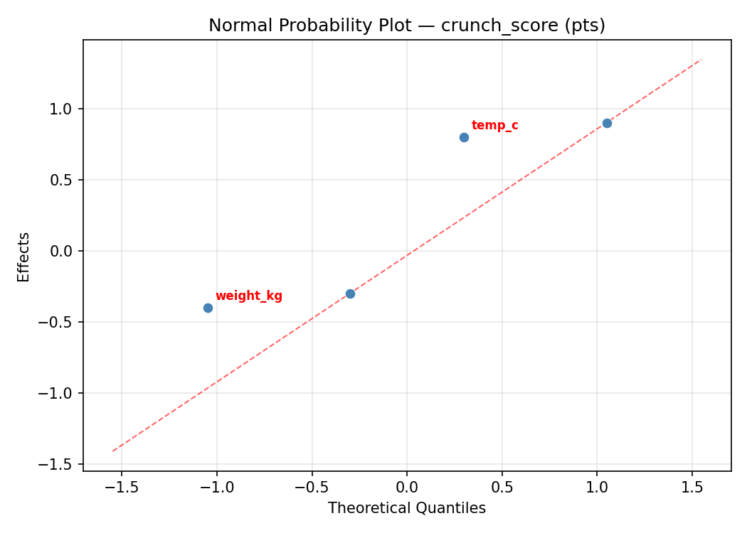
Normal Probability Plot of Effects
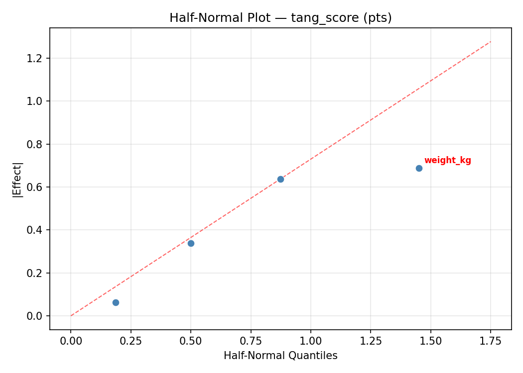
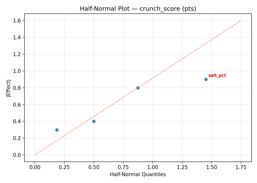
Half-Normal Plot of Effects
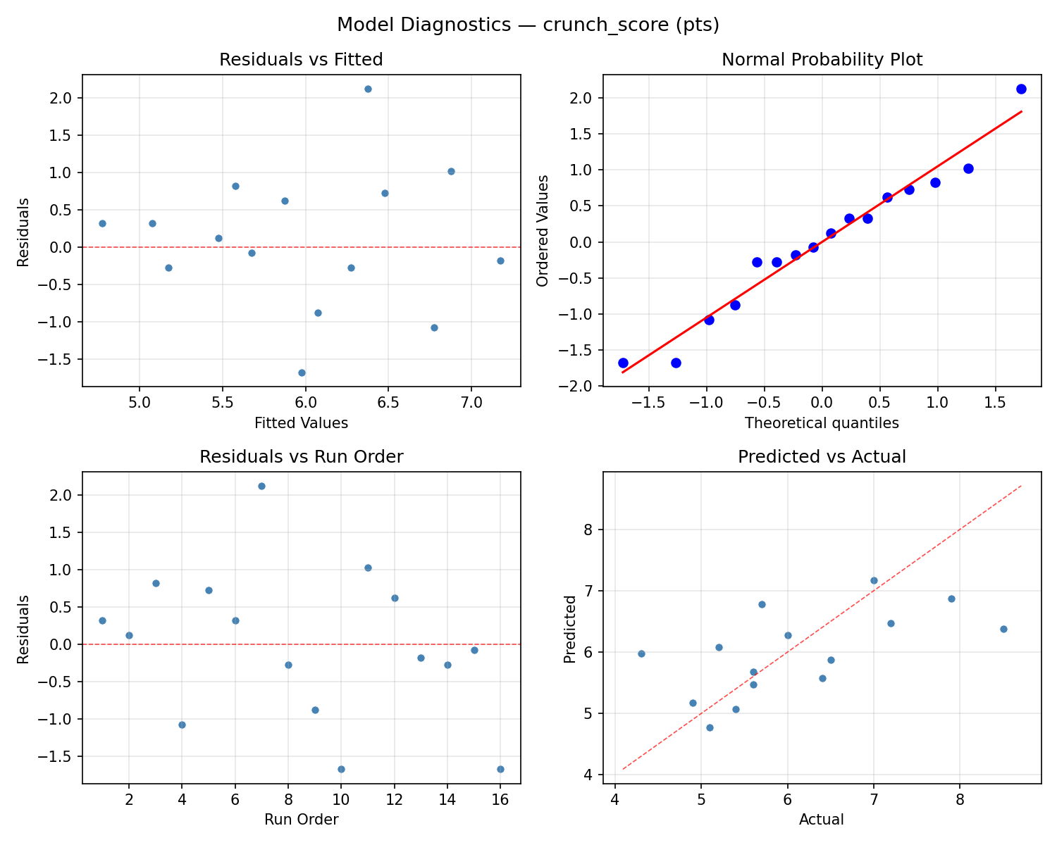
Model Diagnostics
Response: crunch_score
Top factors: temp_c (42.4%), shred_mm (40.9%), weight_kg (10.6%).
ANOVA
| Source | DF | SS | MS | F | p-value |
|---|
| Source | DF | SS | MS | F | p-value |
| salt_pct | 1 | 0.0400 | 0.0400 | 0.015 | 0.9068 |
| shred_mm | 1 | 1.8225 | 1.8225 | 0.690 | 0.4440 |
| temp_c | 1 | 1.9600 | 1.9600 | 0.742 | 0.4283 |
| weight_kg | 1 | 0.1225 | 0.1225 | 0.046 | 0.8380 |
| salt_pct*shred_mm | 1 | 0.3025 | 0.3025 | 0.115 | 0.7488 |
| salt_pct*temp_c | 1 | 0.2500 | 0.2500 | 0.095 | 0.7707 |
| salt_pct*weight_kg | 1 | 0.2025 | 0.2025 | 0.077 | 0.7929 |
| shred_mm*temp_c | 1 | 0.2025 | 0.2025 | 0.077 | 0.7929 |
| shred_mm*weight_kg | 1 | 0.0000 | 0.0000 | 0.000 | 1.0000 |
| temp_c*weight_kg | 1 | 3.8025 | 3.8025 | 1.440 | 0.2839 |
| Error | 5 | 13.2050 | 2.6410 | | |
| Total | 15 | 21.9100 | 1.4607 | | |
Pareto Chart
Main Effects Plot
Normal Probability Plot of Effects
Half-Normal Plot of Effects
Model Diagnostics
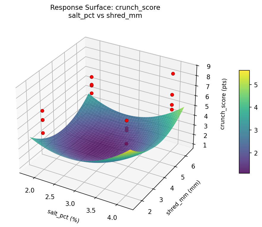
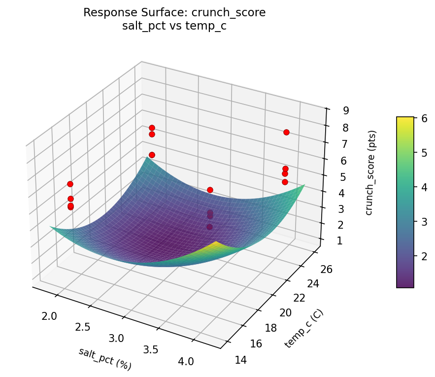
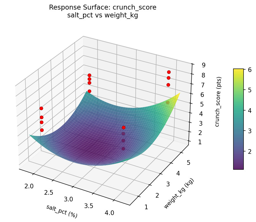
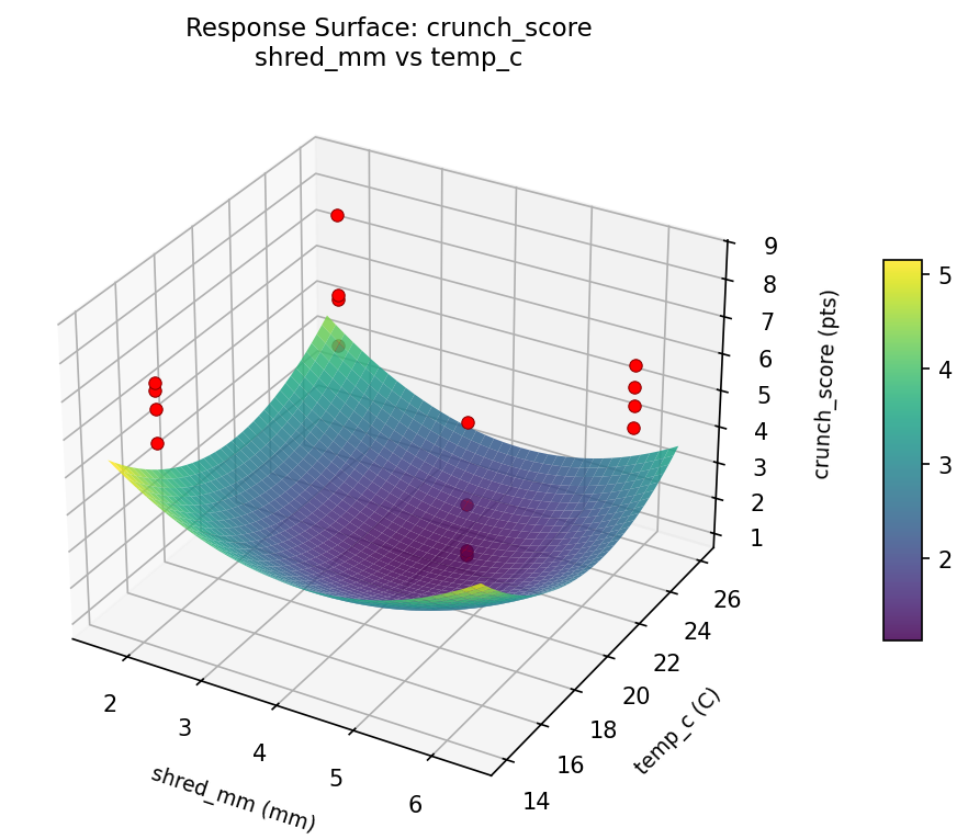
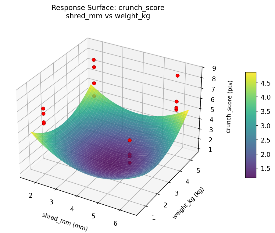
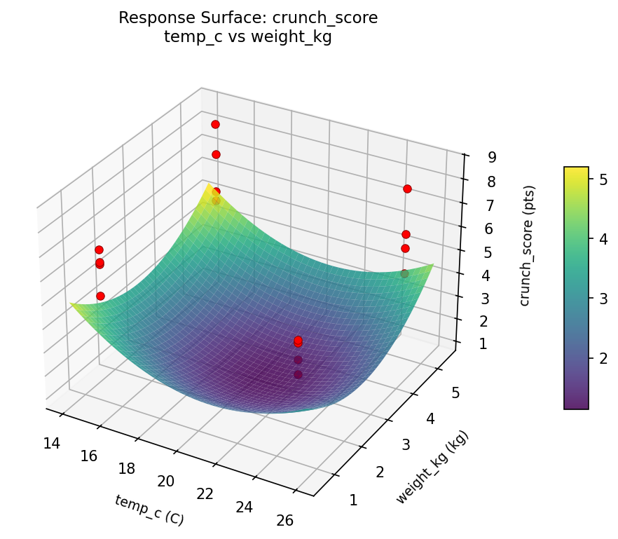
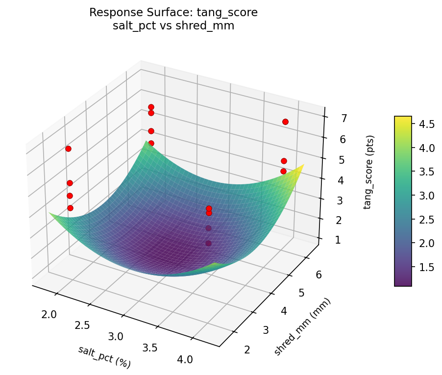
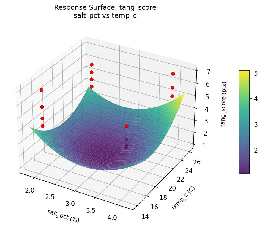
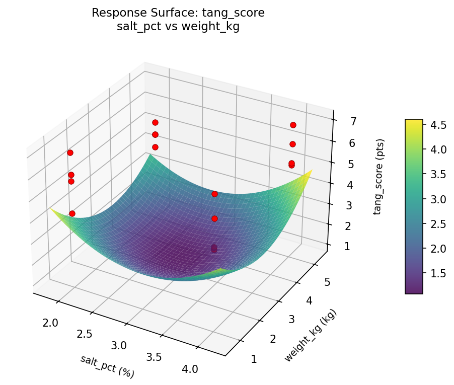
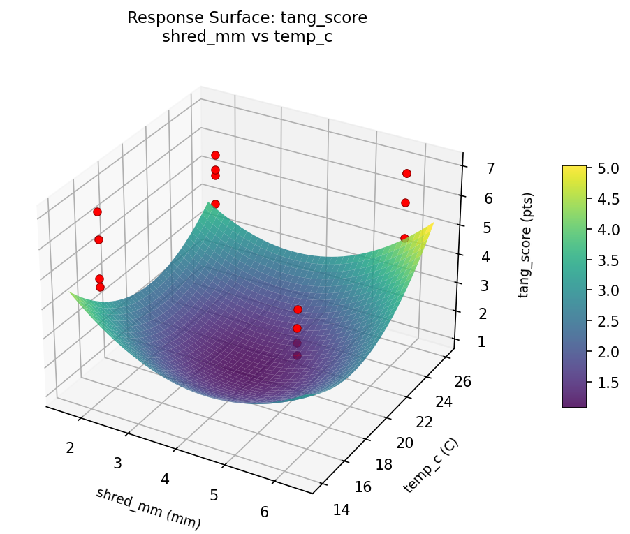
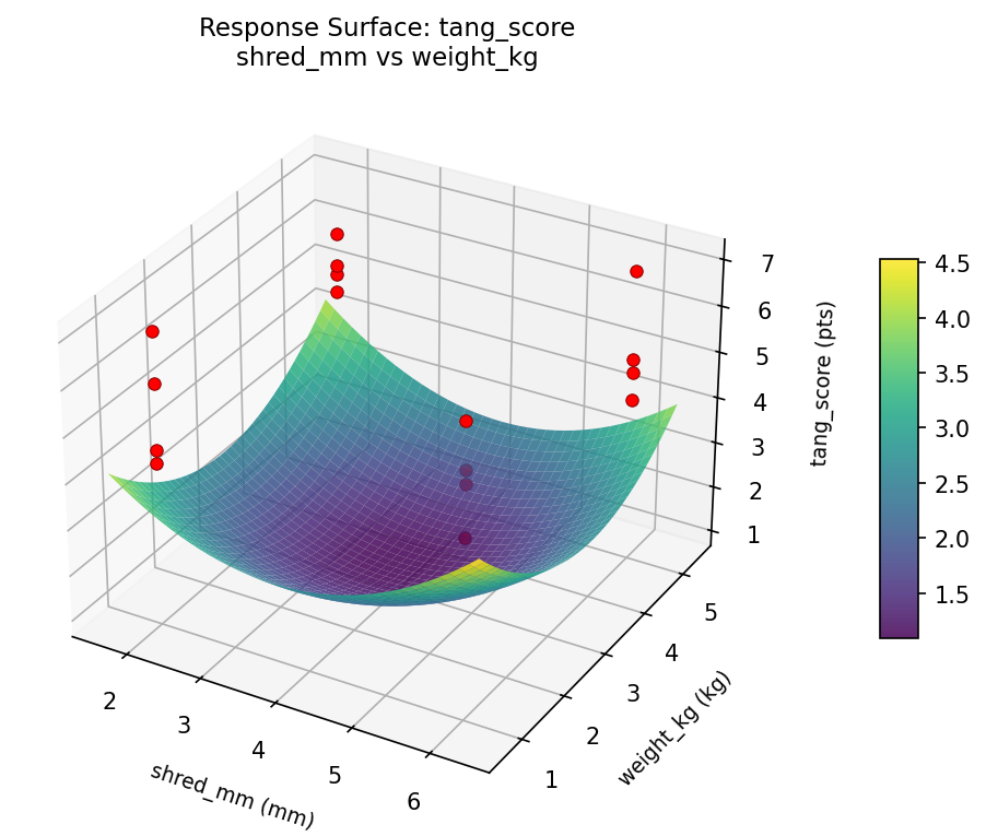
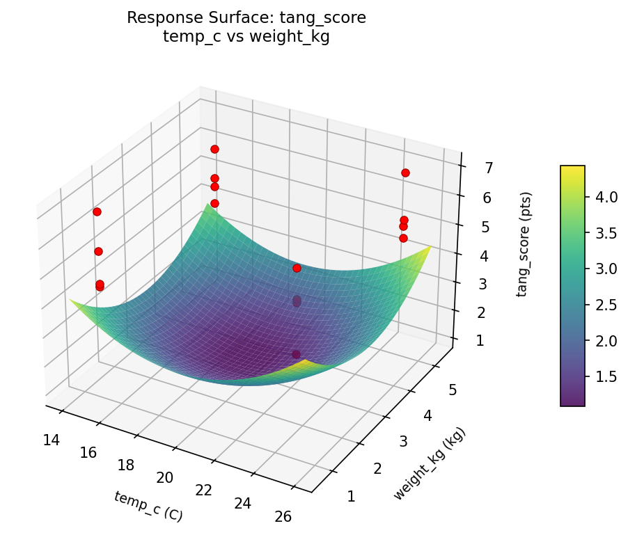
Response Surface Plots
3D surfaces fitted with quadratic RSM. Red dots are observed data points.
crunch score salt pct vs shred mm
crunch score salt pct vs temp c
crunch score salt pct vs weight kg
crunch score shred mm vs temp c
crunch score shred mm vs weight kg
crunch score temp c vs weight kg
tang score salt pct vs shred mm
tang score salt pct vs temp c
tang score salt pct vs weight kg
tang score shred mm vs temp c
tang score shred mm vs weight kg
tang score temp c vs weight kg
Multi-Objective Optimization
When responses compete, Derringer–Suich desirability finds the best compromise.
Each response is scaled to a 0–1 desirability, then combined via a weighted geometric mean.
Overall Desirability
D = 0.7056
Per-Response Desirability
| Response | Weight | Desirability | Predicted | Dir |
|---|
tang_score |
1.5 |
|
7.00 0.9545 7.00 pts |
↑ |
crunch_score |
1.5 |
|
6.50 0.5216 6.50 pts |
↑ |
Recommended Settings
| Factor | Value |
|---|
salt_pct | 4 % |
shred_mm | 2 mm |
temp_c | 15 C |
weight_kg | 1 kg |
Source: from observed run #12
Trade-off Summary
Sacrifice = how much worse than single-objective best.
| Response | Predicted | Best Observed | Sacrifice |
|---|
crunch_score | 6.50 | 8.50 | +2.00 |
Top 3 Runs by Desirability
| Run | D | Factor Settings |
|---|
| #5 | 0.6677 | salt_pct=2, shred_mm=2, temp_c=25, weight_kg=1 |
| #7 | 0.5677 | salt_pct=4, shred_mm=2, temp_c=15, weight_kg=5 |
Model Quality
| Response | R² | Type |
|---|
crunch_score | 0.3671 | linear |
Full Multi-Objective Output
============================================================
MULTI-OBJECTIVE OPTIMIZATION
Method: Derringer-Suich Desirability Function
============================================================
Overall desirability: D = 0.7056
Response Weight Desirability Predicted Direction
---------------------------------------------------------------------
tang_score 1.5 0.9545 7.00 pts ↑
crunch_score 1.5 0.5216 6.50 pts ↑
Recommended settings:
salt_pct = 4 %
shred_mm = 2 mm
temp_c = 15 C
weight_kg = 1 kg
(from observed run #12)
Trade-off summary:
tang_score: 7.00 (best observed: 7.00, sacrifice: +0.00)
crunch_score: 6.50 (best observed: 8.50, sacrifice: +2.00)
Model quality:
tang_score: R² = 0.1955 (linear)
crunch_score: R² = 0.3671 (linear)
Top 3 observed runs by overall desirability:
1. Run #12 (D=0.7056): salt_pct=4, shred_mm=2, temp_c=15, weight_kg=1
2. Run #5 (D=0.6677): salt_pct=2, shred_mm=2, temp_c=25, weight_kg=1
3. Run #7 (D=0.5677): salt_pct=4, shred_mm=2, temp_c=15, weight_kg=5
Full Analysis Output
=== Main Effects: tang_score ===
Factor Effect Std Error % Contribution
--------------------------------------------------------------
salt_pct -0.4625 0.2413 63.8%
shred_mm 0.1375 0.2413 19.0%
weight_kg 0.0875 0.2413 12.1%
temp_c 0.0375 0.2413 5.2%
=== ANOVA Table: tang_score ===
Source DF SS MS F p-value
-----------------------------------------------------------------------------
salt_pct 1 0.8556 0.8556 1.125 0.3374
shred_mm 1 0.0756 0.0756 0.099 0.7653
temp_c 1 0.0056 0.0056 0.007 0.9348
weight_kg 1 0.0306 0.0306 0.040 0.8489
salt_pct*shred_mm 1 0.6006 0.6006 0.790 0.4149
salt_pct*temp_c 1 1.3806 1.3806 1.815 0.2357
salt_pct*weight_kg 1 0.1056 0.1056 0.139 0.7247
shred_mm*temp_c 1 5.1756 5.1756 6.804 0.0478
shred_mm*weight_kg 1 0.0506 0.0506 0.067 0.8067
temp_c*weight_kg 1 1.8906 1.8906 2.486 0.1757
Error 5 3.8031 0.7606
Total 15 13.9744 0.9316
=== Interaction Effects: tang_score ===
Factor A Factor B Interaction % Contribution
------------------------------------------------------------------------
shred_mm temp_c 1.1375 37.0%
temp_c weight_kg 0.6875 22.4%
salt_pct temp_c 0.5875 19.1%
salt_pct shred_mm 0.3875 12.6%
salt_pct weight_kg -0.1625 5.3%
shred_mm weight_kg -0.1125 3.7%
=== Summary Statistics: tang_score ===
salt_pct:
Level N Mean Std Min Max
------------------------------------------------------------
2 8 5.7000 1.1071 4.5000 7.0000
4 8 5.2375 0.8052 4.2000 6.1000
shred_mm:
Level N Mean Std Min Max
------------------------------------------------------------
2 8 5.4000 1.1123 4.2000 7.0000
6 8 5.5375 0.8651 4.2000 7.0000
temp_c:
Level N Mean Std Min Max
------------------------------------------------------------
15 8 5.4500 1.0529 4.2000 7.0000
25 8 5.4875 0.9418 4.2000 7.0000
weight_kg:
Level N Mean Std Min Max
------------------------------------------------------------
1 8 5.4250 0.8396 4.2000 7.0000
5 8 5.5125 1.1344 4.2000 7.0000
=== Main Effects: crunch_score ===
Factor Effect Std Error % Contribution
--------------------------------------------------------------
temp_c -0.7000 0.3021 42.4%
shred_mm -0.6750 0.3021 40.9%
weight_kg 0.1750 0.3021 10.6%
salt_pct -0.1000 0.3021 6.1%
=== ANOVA Table: crunch_score ===
Source DF SS MS F p-value
-----------------------------------------------------------------------------
salt_pct 1 0.0400 0.0400 0.015 0.9068
shred_mm 1 1.8225 1.8225 0.690 0.4440
temp_c 1 1.9600 1.9600 0.742 0.4283
weight_kg 1 0.1225 0.1225 0.046 0.8380
salt_pct*shred_mm 1 0.3025 0.3025 0.115 0.7488
salt_pct*temp_c 1 0.2500 0.2500 0.095 0.7707
salt_pct*weight_kg 1 0.2025 0.2025 0.077 0.7929
shred_mm*temp_c 1 0.2025 0.2025 0.077 0.7929
shred_mm*weight_kg 1 0.0000 0.0000 0.000 1.0000
temp_c*weight_kg 1 3.8025 3.8025 1.440 0.2839
Error 5 13.2050 2.6410
Total 15 21.9100 1.4607
=== Interaction Effects: crunch_score ===
Factor A Factor B Interaction % Contribution
------------------------------------------------------------------------
temp_c weight_kg 0.9750 50.0%
salt_pct shred_mm -0.2750 14.1%
salt_pct temp_c 0.2500 12.8%
salt_pct weight_kg 0.2250 11.5%
shred_mm temp_c -0.2250 11.5%
shred_mm weight_kg 0.0000 0.0%
=== Summary Statistics: crunch_score ===
salt_pct:
Level N Mean Std Min Max
------------------------------------------------------------
2 8 6.0250 1.3156 4.3000 8.5000
4 8 5.9250 1.1805 4.3000 7.9000
shred_mm:
Level N Mean Std Min Max
------------------------------------------------------------
2 8 6.3125 0.8323 5.4000 7.9000
6 8 5.6375 1.4755 4.3000 8.5000
temp_c:
Level N Mean Std Min Max
------------------------------------------------------------
15 8 6.3250 1.2759 5.1000 8.5000
25 8 5.6250 1.1055 4.3000 7.2000
weight_kg:
Level N Mean Std Min Max
------------------------------------------------------------
1 8 5.8875 1.5524 4.3000 8.5000
5 8 6.0625 0.8383 4.9000 7.2000
Optimization Recommendations
=== Optimization: tang_score ===
Direction: maximize
Best observed run: #1
salt_pct = 2
shred_mm = 2
temp_c = 25
weight_kg = 1
Value: 7.0
RSM Model (linear, R² = 0.3741, Adj R² = 0.1465):
Coefficients:
intercept +5.4688
salt_pct -0.3438
shred_mm -0.0688
temp_c -0.4187
weight_kg -0.1688
RSM Model (quadratic, R² = 0.6284, Adj R² = -4.5743):
Coefficients:
intercept +1.0938
salt_pct -0.3438
shred_mm -0.0688
temp_c -0.4187
weight_kg -0.1688
salt_pct*shred_mm +0.3188
salt_pct*temp_c -0.0312
salt_pct*weight_kg -0.2563
shred_mm*temp_c -0.1563
shred_mm*weight_kg +0.1438
temp_c*weight_kg +0.0938
salt_pct^2 +1.0938
shred_mm^2 +1.0938
temp_c^2 +1.0938
weight_kg^2 +1.0938
Curvature analysis:
salt_pct coef=+1.0938 convex (has a minimum)
shred_mm coef=+1.0938 convex (has a minimum)
temp_c coef=+1.0938 convex (has a minimum)
weight_kg coef=+1.0938 convex (has a minimum)
Notable interactions:
salt_pct*shred_mm coef=+0.3188 (synergistic)
Predicted optimum (from linear model, at observed points):
salt_pct = 2
shred_mm = 2
temp_c = 15
weight_kg = 1
Predicted value: 6.4688
Surface optimum (via L-BFGS-B, linear model):
salt_pct = 2
shred_mm = 2
temp_c = 15
weight_kg = 1
Predicted value: 6.4688
Model quality: Weak fit — consider adding center points or using a different design.
Factor importance:
1. temp_c (effect: -0.8, contribution: 41.9%)
2. salt_pct (effect: -0.7, contribution: 34.4%)
3. weight_kg (effect: -0.3, contribution: 16.9%)
4. shred_mm (effect: -0.1, contribution: 6.9%)
=== Optimization: crunch_score ===
Direction: maximize
Best observed run: #7
salt_pct = 2
shred_mm = 2
temp_c = 25
weight_kg = 5
Value: 8.5
RSM Model (linear, R² = 0.1810, Adj R² = -0.1169):
Coefficients:
intercept +5.9750
salt_pct +0.3125
shred_mm +0.0750
temp_c +0.2625
weight_kg +0.2750
RSM Model (quadratic, R² = 0.3658, Adj R² = -8.5128):
Coefficients:
intercept +1.1950
salt_pct +0.3125
shred_mm +0.0750
temp_c +0.2625
weight_kg +0.2750
salt_pct*shred_mm +0.3875
salt_pct*temp_c -0.0250
salt_pct*weight_kg -0.2875
shred_mm*temp_c -0.1125
shred_mm*weight_kg -0.0750
temp_c*weight_kg -0.0375
salt_pct^2 +1.1950
shred_mm^2 +1.1950
temp_c^2 +1.1950
weight_kg^2 +1.1950
Curvature analysis:
salt_pct coef=+1.1950 convex (has a minimum)
shred_mm coef=+1.1950 convex (has a minimum)
temp_c coef=+1.1950 convex (has a minimum)
weight_kg coef=+1.1950 convex (has a minimum)
Notable interactions:
salt_pct*shred_mm coef=+0.3875 (synergistic)
Predicted optimum (from linear model, at observed points):
salt_pct = 4
shred_mm = 6
temp_c = 25
weight_kg = 5
Predicted value: 6.9000
Surface optimum (via L-BFGS-B, linear model):
salt_pct = 4
shred_mm = 6
temp_c = 25
weight_kg = 5
Predicted value: 6.9000
Model quality: Weak fit — consider adding center points or using a different design.
Factor importance:
1. salt_pct (effect: 0.6, contribution: 33.8%)
2. weight_kg (effect: 0.5, contribution: 29.7%)
3. temp_c (effect: 0.5, contribution: 28.4%)
4. shred_mm (effect: 0.1, contribution: 8.1%)