Coral Reef Fragment Restoration

Summary

This experiment investigates coral reef fragment restoration. Box-Behnken design to maximize coral growth rate and survival by tuning fragment size, depth placement, and spacing.

The design varies 3 factors: fragment cm (cm), ranging from 3 to 10, depth m (m), ranging from 3 to 15, and spacing cm (cm), ranging from 10 to 40. The goal is to optimize 2 responses: growth cm yr (cm/yr) (maximize) and survival pct (%) (maximize). Fixed conditions held constant across all runs include species = acropora, substrate = ceramic_disc.

A Box-Behnken design was chosen because it efficiently fits quadratic models with 3 continuous factors while avoiding extreme corner combinations — requiring only 15 runs instead of the 8 needed for a full factorial at two levels.

Quadratic response surface models were fitted to capture potential curvature and factor interactions. The RSM contour plots below visualize how pairs of factors jointly affect each response.

Key Findings

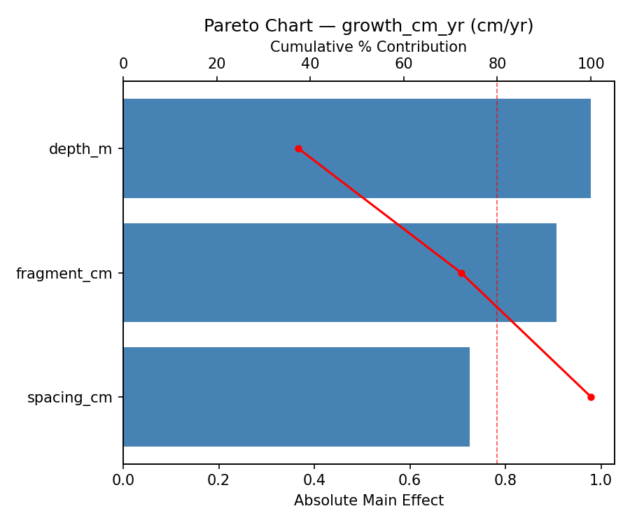
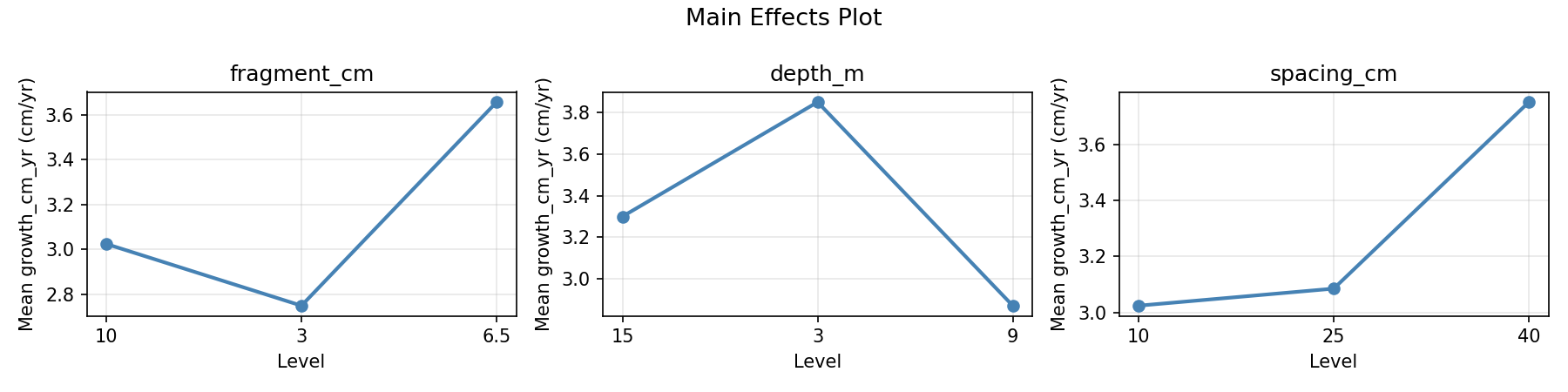
For growth cm yr, the most influential factors were fragment cm (50.7%), depth m (30.3%), spacing cm (19.0%). The best observed value was 4.6 (at fragment cm = 6.5, depth m = 15, spacing cm = 10).

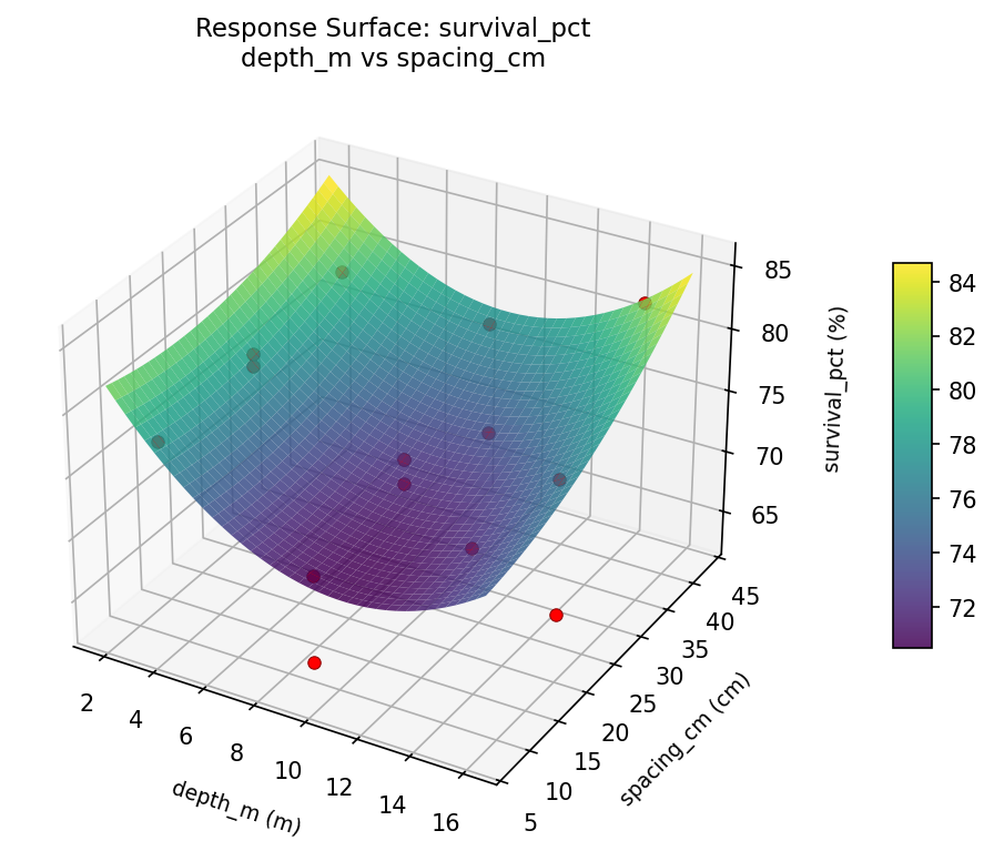
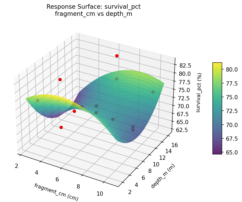
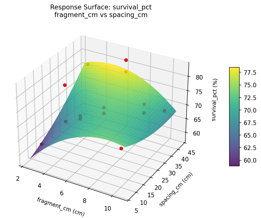
For survival pct, the most influential factors were fragment cm (63.7%), depth m (25.4%), spacing cm (11.0%). The best observed value was 83.0 (at fragment cm = 6.5, depth m = 15, spacing cm = 10).

Recommended Next Steps

Run confirmation experiments at the predicted optimal settings to validate the model.
Consider whether any fixed factors should be varied in a future study.

Experimental Setup

Factors

Factor	Low	High	Unit
`fragment_cm`	3	10	cm
`depth_m`	3	15	m
`spacing_cm`	10	40	cm

Fixed: species = acropora, substrate = ceramic_disc

Responses

Response	Direction	Unit
`growth_cm_yr`	↑ maximize	cm/yr
`survival_pct`	↑ maximize	%

Configuration

use_cases/251_coral_reef_restoration/config.json

{
  "metadata": {
    "name": "Coral Reef Fragment Restoration",
    "description": "Box-Behnken design to maximize coral growth rate and survival by tuning fragment size, depth placement, and spacing"
  },
  "factors": [
    {
      "name": "fragment_cm",
      "levels": [
        "3",
        "10"
      ],
      "type": "continuous",
      "unit": "cm"
    },
    {
      "name": "depth_m",
      "levels": [
        "3",
        "15"
      ],
      "type": "continuous",
      "unit": "m"
    },
    {
      "name": "spacing_cm",
      "levels": [
        "10",
        "40"
      ],
      "type": "continuous",
      "unit": "cm"
    }
  ],
  "fixed_factors": {
    "species": "acropora",
    "substrate": "ceramic_disc"
  },
  "responses": [
    {
      "name": "growth_cm_yr",
      "optimize": "maximize",
      "unit": "cm/yr"
    },
    {
      "name": "survival_pct",
      "optimize": "maximize",
      "unit": "%"
    }
  ],
  "settings": {
    "operation": "box_behnken",
    "test_script": "use_cases/251_coral_reef_restoration/sim.sh"
  }
}

Experimental Matrix

The Box-Behnken Design produces 15 runs. Each row is one experiment with specific factor settings.

Run	`fragment_cm`	`depth_m`	`spacing_cm`
1	6.5	3	10
2	6.5	9	25
3	10	9	40
4	10	9	10
5	6.5	9	25
6	6.5	9	25
7	3	9	40
8	10	3	25
9	6.5	3	40
10	10	15	25
11	3	9	10
12	6.5	15	40
13	3	3	25
14	3	15	25
15	6.5	15	10

Step-by-Step Workflow

1

Preview the design

Terminal

$ doe info --config use_cases/251_coral_reef_restoration/config.json

2

Generate the runner script

Terminal

$ doe generate --config use_cases/251_coral_reef_restoration/config.json \
    --output use_cases/251_coral_reef_restoration/results/run.sh --seed 42

3

Execute the experiments

Terminal

$ bash use_cases/251_coral_reef_restoration/results/run.sh

4

Analyze results

Terminal

$ doe analyze --config use_cases/251_coral_reef_restoration/config.json

5

Get optimization recommendations

Terminal

$ doe optimize --config use_cases/251_coral_reef_restoration/config.json

6

Multi-objective optimization

With 2 competing responses, use --multi to find the best compromise via Derringer–Suich desirability.

Terminal

$ doe optimize --config use_cases/251_coral_reef_restoration/config.json --multi

7

Generate the HTML report

Terminal

$ doe report --config use_cases/251_coral_reef_restoration/config.json \
    --output use_cases/251_coral_reef_restoration/results/report.html

Features Exercised

Feature	Value
Design type	`box_behnken`
Factor types	`continuous` (all 3)
Arg style	`double-dash`
Responses	2 (growth_cm_yr ↑, survival_pct ↑)
Total runs	15

Analysis Results

Generated from actual experiment runs using the DOE Helper Tool.

Response: growth_cm_yr

Top factors: fragment_cm (50.7%), depth_m (30.3%), spacing_cm (19.0%).

ANOVA

Source	DF	SS	MS	F	p-value
Source	DF	SS	MS	F	p-value
fragment_cm	2	3.1288	1.5644	3.785	0.0697
depth_m	2	0.9330	0.4665	1.129	0.3700
spacing_cm	2	0.4802	0.2401	0.581	0.5814
Lack	of	Fit	6	3.3687	0.5614
Pure	Error	2	0.8267
Error	8	4.1953	0.4133
Total	14	8.7373	0.6241

Pareto Chart

Main Effects Plot

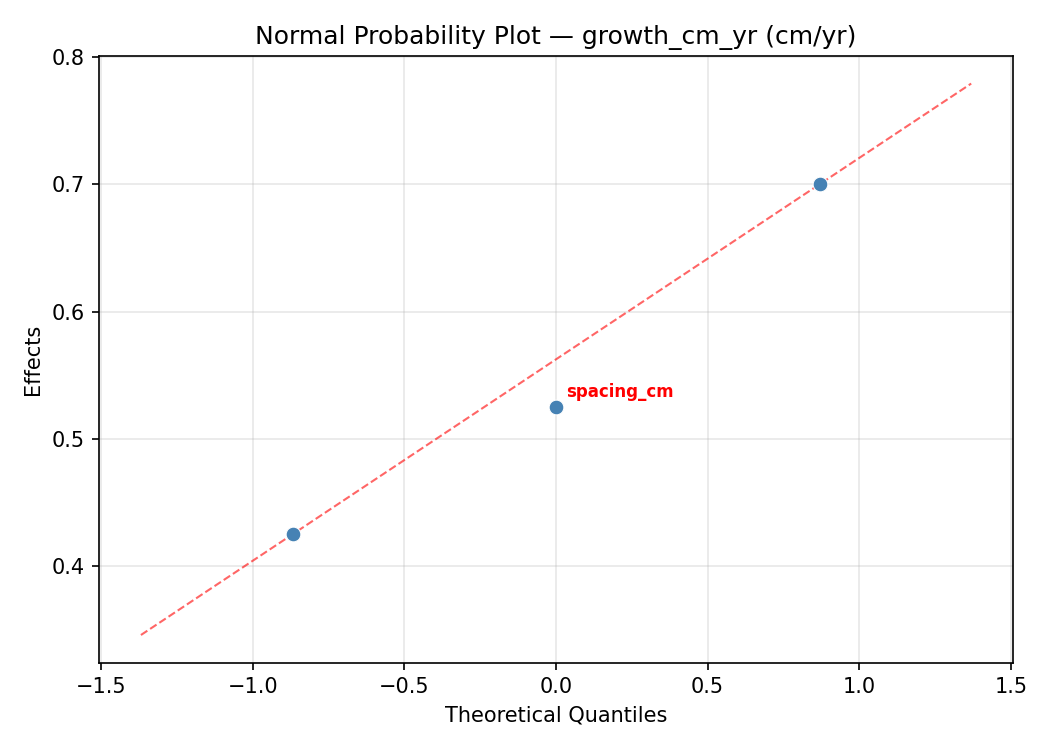
Normal Probability Plot of Effects

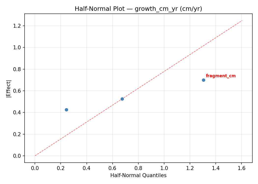
Normal probability plot for growth_cm_yr

Half-Normal Plot of Effects

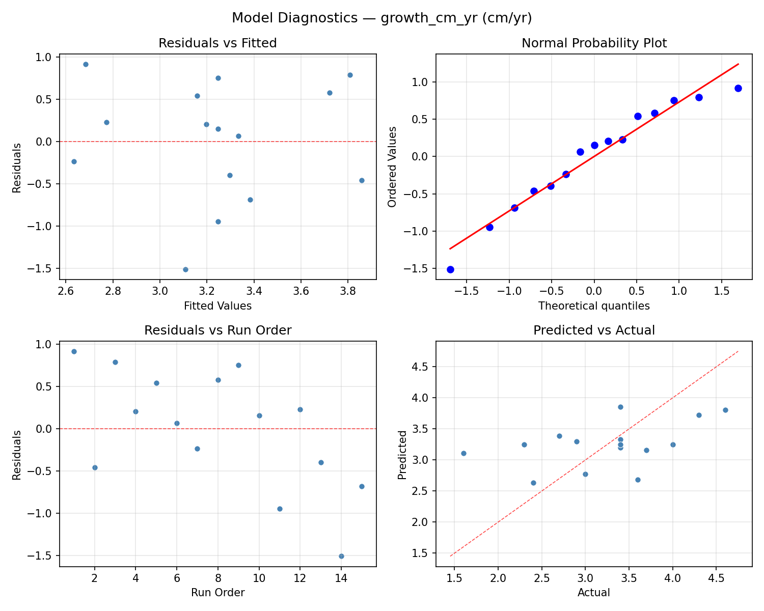
Model Diagnostics

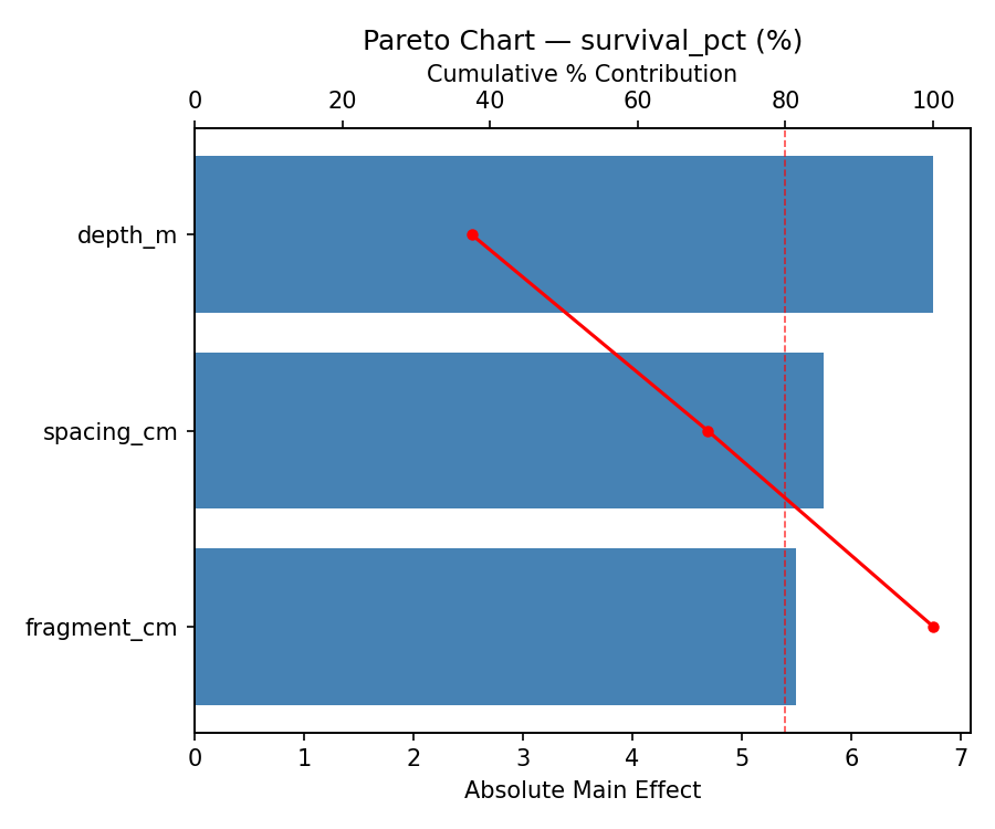
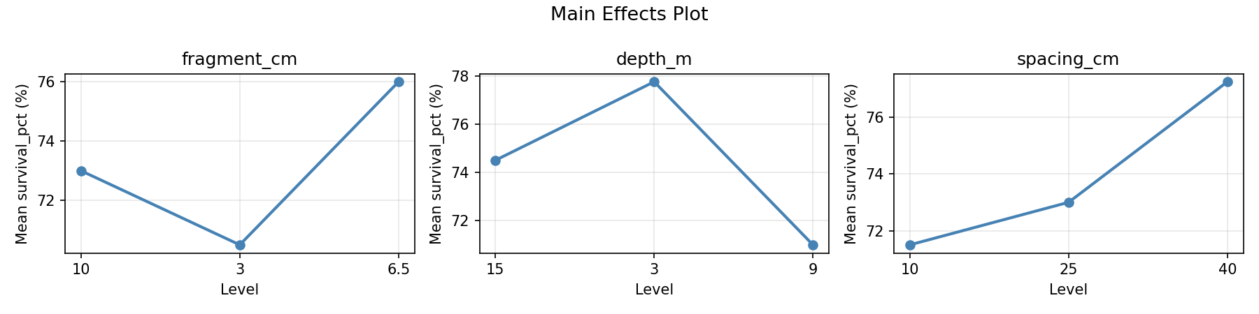
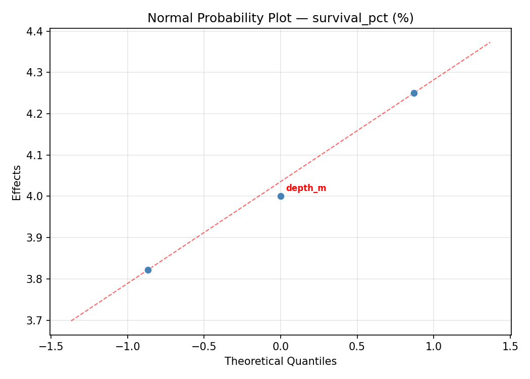
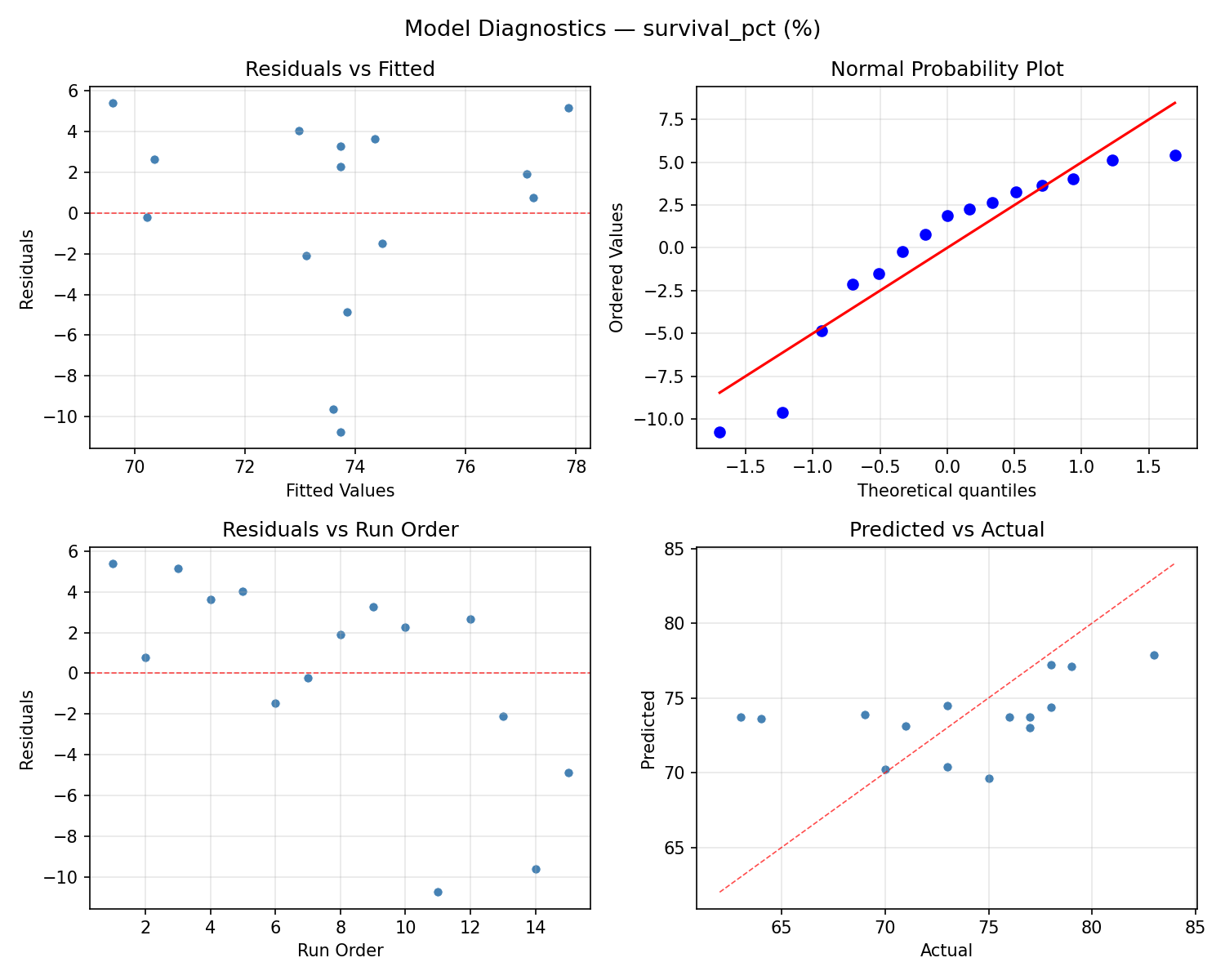
Response: survival_pct

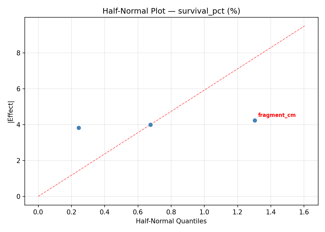
Top factors: fragment_cm (63.7%), depth_m (25.4%), spacing_cm (11.0%).

ANOVA

Source	DF	SS	MS	F	p-value
Source	DF	SS	MS	F	p-value
fragment_cm	2	166.2190	83.1095	5.088	0.0375
depth_m	2	27.7548	13.8774	0.850	0.4628
spacing_cm	2	5.3262	2.6631	0.163	0.8523
Lack	of	Fit	6	200.9667	33.4944
Pure	Error	2	32.6667
Error	8	233.6333	16.3333
Total	14	432.9333	30.9238

Pareto Chart

Main Effects Plot

Normal Probability Plot of Effects

Normal probability plot for survival_pct

Half-Normal Plot of Effects

Model Diagnostics

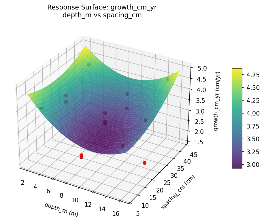
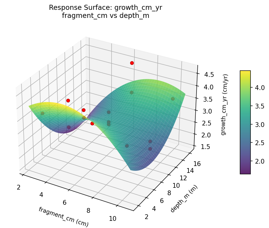
Response Surface Plots

3D surfaces fitted with quadratic RSM. Red dots are observed data points.

growth cm yr depth m vs spacing cm

growth cm yr fragment cm vs depth m

growth cm yr fragment cm vs spacing cm

survival pct depth m vs spacing cm

survival pct fragment cm vs depth m

survival pct fragment cm vs spacing cm

Multi-Objective Optimization

When responses compete, Derringer–Suich desirability finds the best compromise. Each response is scaled to a 0–1 desirability, then combined via a weighted geometric mean.

Overall Desirability

D = 0.9545

Per-Response Desirability

Response	Weight	Desirability	Predicted	Dir
`growth_cm_yr`	1.5	0.9545	4.60 0.9545 4.60 cm/yr	↑
`survival_pct`	2.0	0.9545	83.00 0.9545 83.00 %	↑

Recommended Settings

Factor	Value
`fragment_cm`	6.5 cm
`depth_m`	15 m
`spacing_cm`	10 cm

Source: from observed run #3

Trade-off Summary

Sacrifice = how much worse than single-objective best.

Response	Predicted	Best Observed	Sacrifice
`survival_pct`	83.00	83.00	+0.00

Top 3 Runs by Desirability

Run	D	Factor Settings
#8	0.8105	fragment_cm=3, depth_m=3, spacing_cm=25
#9	0.7194	fragment_cm=3, depth_m=15, spacing_cm=25

Model Quality

Response	R²	Type
`survival_pct`	0.8077	quadratic

Full Multi-Objective Output

doe optimize --multi
============================================================
MULTI-OBJECTIVE OPTIMIZATION
Method: Derringer-Suich Desirability Function
============================================================

Overall desirability: D = 0.9545

Response                  Weight Desirability    Predicted  Direction
---------------------------------------------------------------------
growth_cm_yr                 1.5       0.9545        4.60 cm/yr   ↑
survival_pct                 2.0       0.9545       83.00 %   ↑

Recommended settings:
  fragment_cm = 6.5 cm
  depth_m = 15 m
  spacing_cm = 10 cm
  (from observed run #3)

Trade-off summary:
  growth_cm_yr: 4.60 (best observed: 4.60, sacrifice: +0.00)
  survival_pct: 83.00 (best observed: 83.00, sacrifice: +0.00)

Model quality:
  growth_cm_yr: R² = 0.4226 (linear)
  survival_pct: R² = 0.8077 (quadratic)

Top 3 observed runs by overall desirability:
  1. Run #3 (D=0.9545): fragment_cm=6.5, depth_m=15, spacing_cm=10
  2. Run #8 (D=0.8105): fragment_cm=3, depth_m=3, spacing_cm=25
  3. Run #9 (D=0.7194): fragment_cm=3, depth_m=15, spacing_cm=25

Full Analysis Output

doe analyze
=== Main Effects: growth_cm_yr ===
Factor                   Effect    Std Error   % Contribution
--------------------------------------------------------------
fragment_cm              1.0857       0.2040            50.7%
depth_m                  0.6500       0.2040            30.3%
spacing_cm               0.4071       0.2040            19.0%

=== ANOVA Table: growth_cm_yr ===
Source                      DF           SS           MS          F    p-value
-----------------------------------------------------------------------------
fragment_cm                  2       3.1288       1.5644      3.785     0.0697
depth_m                      2       0.9330       0.4665      1.129     0.3700
spacing_cm                   2       0.4802       0.2401      0.581     0.5814
Lack of Fit                  6       3.3687       0.5614      1.358     0.4823
Pure Error                   2       0.8267       0.4133
Error                        8       4.1953       0.4133
Total                       14       8.7373       0.6241

=== Summary Statistics: growth_cm_yr ===

fragment_cm:
  Level               N       Mean        Std        Min        Max
  ------------------------------------------------------------
  10                  4     3.4000     0.6377     2.9000     4.3000
  3                   4     2.5000     0.8756     1.6000     3.7000
  6.5                 7     3.5857     0.5900     2.7000     4.6000

depth_m:
  Level               N       Mean        Std        Min        Max
  ------------------------------------------------------------
  15                  4     3.5000     0.8832     2.3000     4.3000
  3                   4     2.8500     0.4203     2.4000     3.4000
  9                   7     3.3286     0.9069     1.6000     4.6000

spacing_cm:
  Level               N       Mean        Std        Min        Max
  ------------------------------------------------------------
  10                  4     3.3500     0.6028     2.7000     4.0000
  25                  7     3.3571     0.8886     2.3000     4.6000
  40                  4     2.9500     0.9000     1.6000     3.4000

=== Main Effects: survival_pct ===
Factor                   Effect    Std Error   % Contribution
--------------------------------------------------------------
fragment_cm              8.0714       1.4358            63.7%
depth_m                  3.2143       1.4358            25.4%
spacing_cm               1.3929       1.4358            11.0%

=== ANOVA Table: survival_pct ===
Source                      DF           SS           MS          F    p-value
-----------------------------------------------------------------------------
fragment_cm                  2     166.2190      83.1095      5.088     0.0375
depth_m                      2      27.7548      13.8774      0.850     0.4628
spacing_cm                   2       5.3262       2.6631      0.163     0.8523
Lack of Fit                  6     200.9667      33.4944      2.051     0.3635
Pure Error                   2      32.6667      16.3333
Error                        8     233.6333      16.3333
Total                       14     432.9333      30.9238

=== Summary Statistics: survival_pct ===

fragment_cm:
  Level               N       Mean        Std        Min        Max
  ------------------------------------------------------------
  10                  4    74.0000     3.4641    71.0000    79.0000
  3                   4    68.5000     6.4550    63.0000    77.0000
  6.5                 7    76.5714     4.1975    69.0000    83.0000

depth_m:
  Level               N       Mean        Std        Min        Max
  ------------------------------------------------------------
  15                  4    74.2500     7.5443    63.0000    79.0000
  3                   4    71.5000     3.1091    69.0000    76.0000
  9                   7    74.7143     5.8513    64.0000    83.0000

spacing_cm:
  Level               N       Mean        Std        Min        Max
  ------------------------------------------------------------
  10                  4    74.0000     3.8297    69.0000    77.0000
  25                  7    74.1429     6.6940    63.0000    83.0000
  40                  4    72.7500     6.1847    64.0000    78.0000

Optimization Recommendations

doe optimize
=== Optimization: growth_cm_yr ===
Direction: maximize

Best observed run: #3
  fragment_cm = 6.5
  depth_m = 15
  spacing_cm = 10
  Value: 4.6

RSM Model (linear, R² = 0.3024, Adj R² = 0.1122):
  Coefficients:
    intercept                      +3.2467
    fragment_cm                    +0.0375
    depth_m                        +0.1625
    spacing_cm                     -0.5500

RSM Model (quadratic, R² = 0.8776, Adj R² = 0.6574):
  Coefficients:
    intercept                      +3.4667
    fragment_cm                    +0.0375
    depth_m                        +0.1625
    spacing_cm                     -0.5500
    fragment_cm*depth_m            +0.5250
    fragment_cm*spacing_cm         -0.2000
    depth_m*spacing_cm             -0.5000
    fragment_cm^2                  -0.7458
    depth_m^2                      -0.0458
    spacing_cm^2                   +0.3792

  Curvature analysis:
    fragment_cm                    coef=-0.7458  concave (has a maximum)
    spacing_cm                     coef=+0.3792  convex (has a minimum)
    depth_m                        coef=-0.0458  negligible curvature

  Notable interactions:
    fragment_cm*depth_m            coef=+0.5250  (synergistic)
    depth_m*spacing_cm             coef=-0.5000  (antagonistic)

  Predicted optimum (from quadratic model, at observed points):
    fragment_cm = 6.5
    depth_m = 15
    spacing_cm = 10
    Predicted value: 5.0125

  Surface optimum (via L-BFGS-B, quadratic model):
    fragment_cm = 8.28911
    depth_m = 15
    spacing_cm = 10
    Predicted value: 5.2074

  Model quality: Good fit — general trends are captured, some noise remains.

Factor importance:
  1. spacing_cm  (effect: 1.1, contribution: 49.3%)
  2. fragment_cm  (effect: 0.8, contribution: 36.2%)
  3. depth_m  (effect: 0.3, contribution: 14.6%)

=== Optimization: survival_pct ===
Direction: maximize

Best observed run: #3
  fragment_cm = 6.5
  depth_m = 15
  spacing_cm = 10
  Value: 83.0

RSM Model (linear, R² = 0.3551, Adj R² = 0.1793):
  Coefficients:
    intercept                      +73.7333
    fragment_cm                    +1.6250
    depth_m                        +1.2500
    spacing_cm                     -3.8750

RSM Model (quadratic, R² = 0.8974, Adj R² = 0.7127):
  Coefficients:
    intercept                      +76.3333
    fragment_cm                    +1.6250
    depth_m                        +1.2500
    spacing_cm                     -3.8750
    fragment_cm*depth_m            +4.5000
    fragment_cm*spacing_cm         +0.2500
    depth_m*spacing_cm             -3.0000
    fragment_cm^2                  -5.5417
    depth_m^2                      +0.2083
    spacing_cm^2                   +0.4583

  Curvature analysis:
    fragment_cm                    coef=-5.5417  concave (has a maximum)
    spacing_cm                     coef=+0.4583  convex (has a minimum)
    depth_m                        coef=+0.2083  convex (has a minimum)

  Notable interactions:
    fragment_cm*depth_m            coef=+4.5000  (synergistic)
    depth_m*spacing_cm             coef=-3.0000  (antagonistic)

  Predicted optimum (from quadratic model, at observed points):
    fragment_cm = 6.5
    depth_m = 15
    spacing_cm = 10
    Predicted value: 85.1250

  Surface optimum (via L-BFGS-B, quadratic model):
    fragment_cm = 8.35526
    depth_m = 15
    spacing_cm = 10
    Predicted value: 86.6821

  Model quality: Good fit — general trends are captured, some noise remains.

Factor importance:
  1. spacing_cm  (effect: 7.8, contribution: 44.4%)
  2. fragment_cm  (effect: 7.2, contribution: 41.3%)
  3. depth_m  (effect: 2.5, contribution: 14.3%)

Run	`fragment_cm`	`depth_m`	`spacing_cm`
1	6.5	3	10
2	6.5	9	25
3	10	9	40
4	10	9	10
5	6.5	9	25
6	6.5	9	25
7	3	9	40
8	10	3	25
9	6.5	3	40
10	10	15	25
11	3	9	10
12	6.5	15	40
13	3	3	25
14	3	15	25
15	6.5	15	10

Run	`fragment_cm`	`depth_m`	`spacing_cm`
1	6.5	3	10
2	6.5	9	25
3	10	9	40
4	10	9	10
5	6.5	9	25
6	6.5	9	25
7	3	9	40
8	10	3	25
9	6.5	3	40
10	10	15	25
11	3	9	10
12	6.5	15	40
13	3	3	25
14	3	15	25
15	6.5	15	10

Run	`fragment_cm`	`depth_m`	`spacing_cm`
1	6.5	3	10
2	6.5	9	25
3	10	9	40
4	10	9	10
5	6.5	9	25
6	6.5	9	25
7	3	9	40
8	10	3	25
9	6.5	3	40
10	10	15	25
11	3	9	10
12	6.5	15	40
13	3	3	25
14	3	15	25
15	6.5	15	10