Summary
This experiment investigates model rocket flight optimization. Box-Behnken design to maximize apogee altitude and minimize drift by tuning motor impulse, fin area, and nose cone shape factor.
The design varies 3 factors: impulse ns (Ns), ranging from 5 to 40, fin area cm2 (cm2), ranging from 20 to 80, and nose fineness (ratio), ranging from 3 to 7. The goal is to optimize 2 responses: apogee m (m) (maximize) and drift m (m) (minimize). Fixed conditions held constant across all runs include body diam = 25mm, recovery = parachute.
A Box-Behnken design was chosen because it efficiently fits quadratic models with 3 continuous factors while avoiding extreme corner combinations — requiring only 15 runs instead of the 8 needed for a full factorial at two levels.
Quadratic response surface models were fitted to capture potential curvature and factor interactions. The RSM contour plots below visualize how pairs of factors jointly affect each response.
Key Findings
For apogee m, the most influential factors were impulse ns (36.7%), fin area cm2 (32.5%), nose fineness (30.8%). The best observed value was 242.0 (at impulse ns = 22.5, fin area cm2 = 50, nose fineness = 5).
For drift m, the most influential factors were fin area cm2 (76.1%), impulse ns (21.8%), nose fineness (2.1%). The best observed value was 30.0 (at impulse ns = 22.5, fin area cm2 = 80, nose fineness = 7).
Recommended Next Steps
- Run confirmation experiments at the predicted optimal settings to validate the model.
- Consider whether any fixed factors should be varied in a future study.
Experimental Setup
Factors
| Factor | Low | High | Unit |
|---|
impulse_ns | 5 | 40 | Ns |
fin_area_cm2 | 20 | 80 | cm2 |
nose_fineness | 3 | 7 | ratio |
Fixed: body_diam = 25mm, recovery = parachute
Responses
| Response | Direction | Unit |
|---|
apogee_m | ↑ maximize | m |
drift_m | ↓ minimize | m |
Configuration
{
"metadata": {
"name": "Model Rocket Flight Optimization",
"description": "Box-Behnken design to maximize apogee altitude and minimize drift by tuning motor impulse, fin area, and nose cone shape factor"
},
"factors": [
{
"name": "impulse_ns",
"levels": [
"5",
"40"
],
"type": "continuous",
"unit": "Ns"
},
{
"name": "fin_area_cm2",
"levels": [
"20",
"80"
],
"type": "continuous",
"unit": "cm2"
},
{
"name": "nose_fineness",
"levels": [
"3",
"7"
],
"type": "continuous",
"unit": "ratio"
}
],
"fixed_factors": {
"body_diam": "25mm",
"recovery": "parachute"
},
"responses": [
{
"name": "apogee_m",
"optimize": "maximize",
"unit": "m"
},
{
"name": "drift_m",
"optimize": "minimize",
"unit": "m"
}
],
"settings": {
"operation": "box_behnken",
"test_script": "use_cases/261_model_rocket_flight/sim.sh"
}
}
Experimental Matrix
The Box-Behnken Design produces 15 runs. Each row is one experiment with specific factor settings.
| Run | impulse_ns | fin_area_cm2 | nose_fineness |
|---|
| 1 | 22.5 | 20 | 3 |
| 2 | 22.5 | 50 | 5 |
| 3 | 40 | 50 | 7 |
| 4 | 40 | 50 | 3 |
| 5 | 22.5 | 50 | 5 |
| 6 | 22.5 | 50 | 5 |
| 7 | 5 | 50 | 7 |
| 8 | 40 | 20 | 5 |
| 9 | 22.5 | 20 | 7 |
| 10 | 40 | 80 | 5 |
| 11 | 5 | 50 | 3 |
| 12 | 22.5 | 80 | 7 |
| 13 | 5 | 20 | 5 |
| 14 | 5 | 80 | 5 |
| 15 | 22.5 | 80 | 3 |
Step-by-Step Workflow
1
Preview the design
$ doe info --config use_cases/261_model_rocket_flight/config.json
2
Generate the runner script
$ doe generate --config use_cases/261_model_rocket_flight/config.json \
--output use_cases/261_model_rocket_flight/results/run.sh --seed 42
3
Execute the experiments
$ bash use_cases/261_model_rocket_flight/results/run.sh
4
Analyze results
$ doe analyze --config use_cases/261_model_rocket_flight/config.json
5
Get optimization recommendations
$ doe optimize --config use_cases/261_model_rocket_flight/config.json
6
Multi-objective optimization
With 2 competing responses, use --multi to find the best compromise via Derringer–Suich desirability.
$ doe optimize --config use_cases/261_model_rocket_flight/config.json --multi
7
Generate the HTML report
$ doe report --config use_cases/261_model_rocket_flight/config.json \
--output use_cases/261_model_rocket_flight/results/report.html
Features Exercised
| Feature | Value |
|---|
| Design type | box_behnken |
| Factor types | continuous (all 3) |
| Arg style | double-dash |
| Responses | 2 (apogee_m ↑, drift_m ↓) |
| Total runs | 15 |
Analysis Results
Generated from actual experiment runs using the DOE Helper Tool.
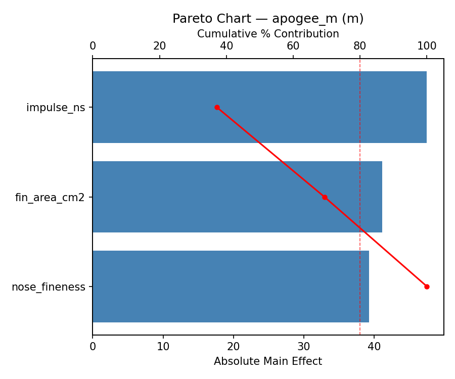
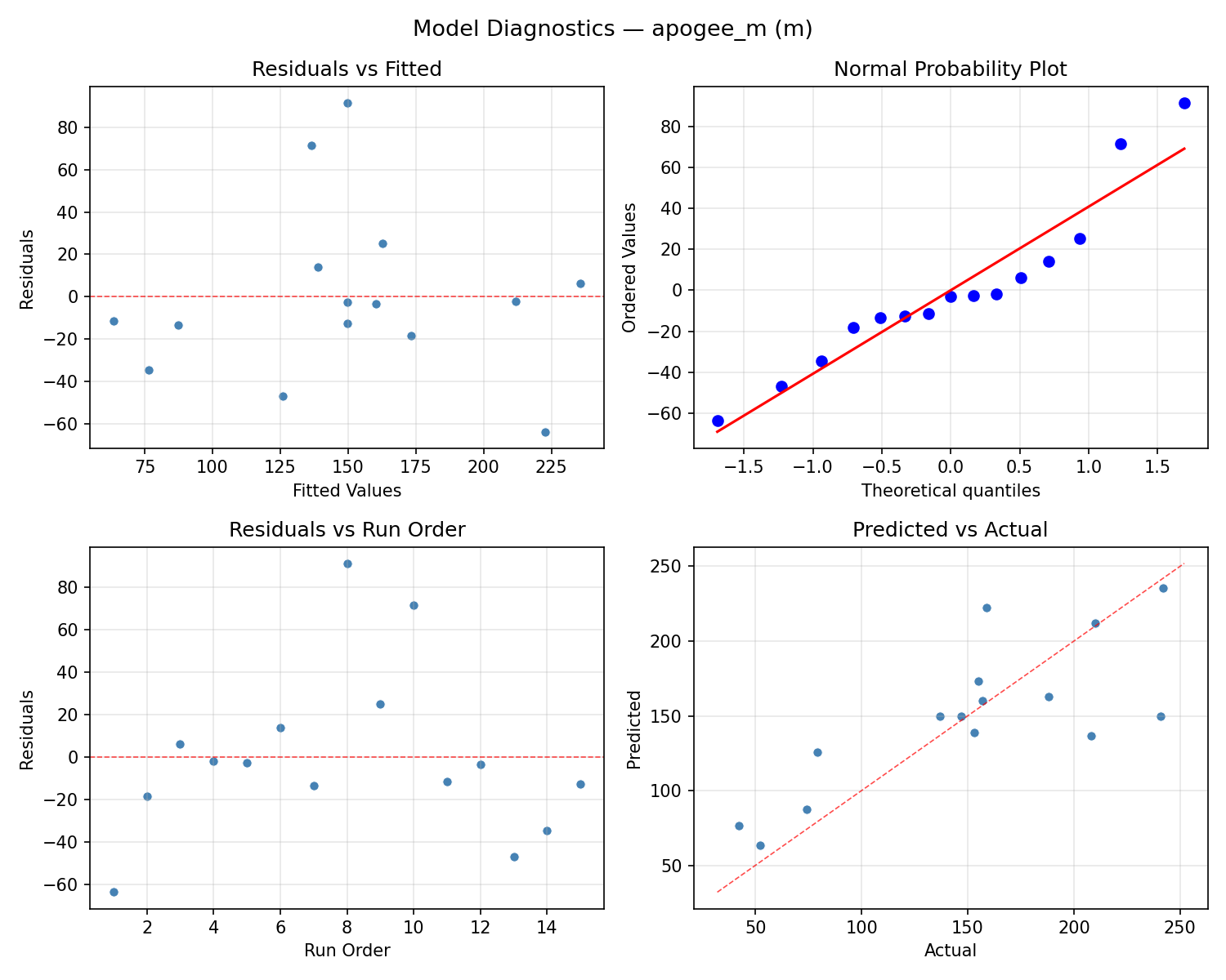
Response: apogee_m
Top factors: impulse_ns (36.7%), fin_area_cm2 (32.5%), nose_fineness (30.8%).
ANOVA
| Source | DF | SS | MS | F | p-value |
|---|
| Source | DF | SS | MS | F | p-value |
| impulse_ns | 2 | 6262.4214 | 3131.2107 | 8.938 | 0.0091 |
| fin_area_cm2 | 2 | 5931.8857 | 2965.9429 | 8.466 | 0.0106 |
| nose_fineness | 2 | 4338.1357 | 2169.0679 | 6.191 | 0.0237 |
| Lack | of | Fit | 6 | 40344.4905 | 6724.0817 |
| Pure | Error | 2 | 700.6667 | | |
| Error | 8 | 41045.1571 | 350.3333 | | |
| Total | 14 | 57577.6000 | 4112.6857 | | |
Pareto Chart
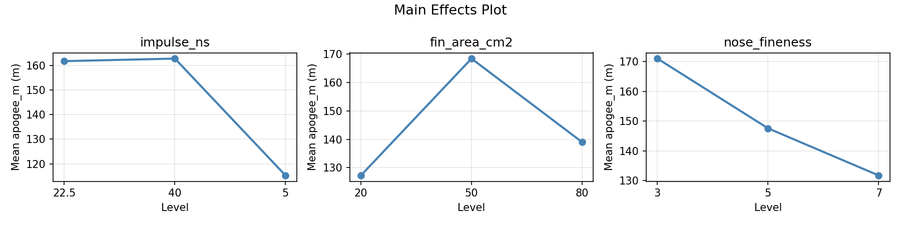
Main Effects Plot
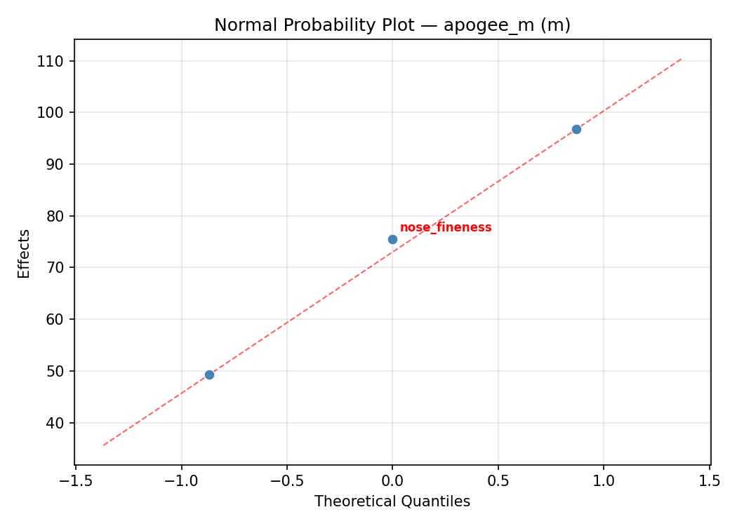
Normal Probability Plot of Effects
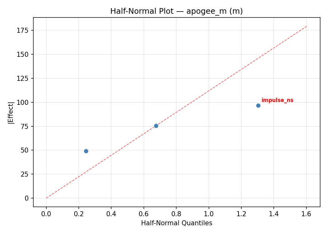
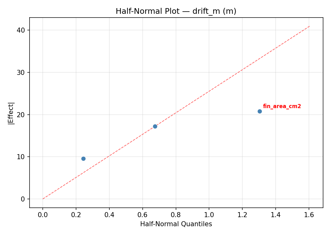
Half-Normal Plot of Effects
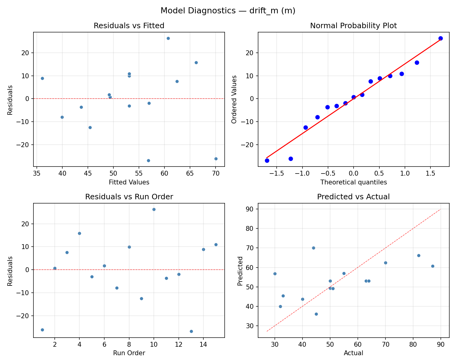
Model Diagnostics
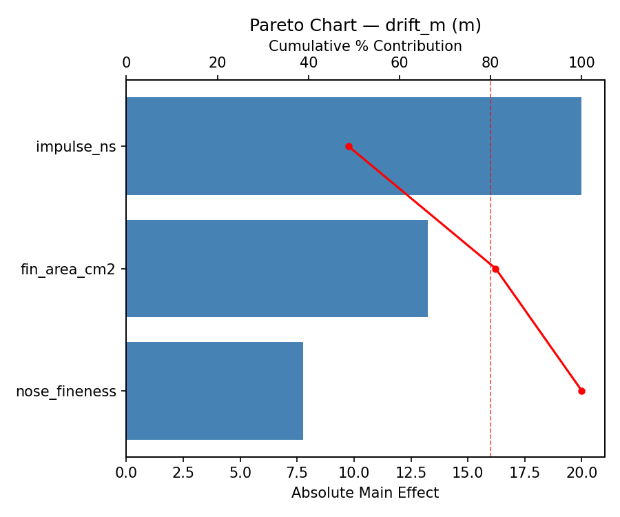
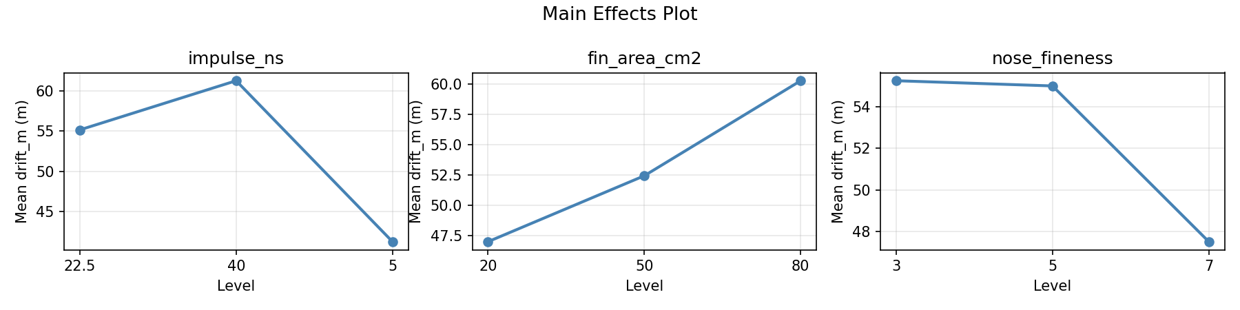
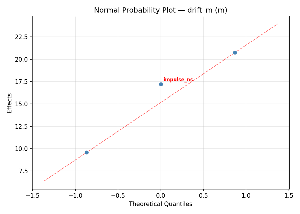
Response: drift_m
Top factors: fin_area_cm2 (76.1%), impulse_ns (21.8%), nose_fineness (2.1%).
ANOVA
| Source | DF | SS | MS | F | p-value |
|---|
| Source | DF | SS | MS | F | p-value |
| impulse_ns | 2 | 47.3262 | 23.6631 | 0.287 | 0.7576 |
| fin_area_cm2 | 2 | 738.4690 | 369.2345 | 4.485 | 0.0494 |
| nose_fineness | 2 | 0.5762 | 0.2881 | 0.003 | 0.9965 |
| Lack | of | Fit | 6 | 3265.8952 | 544.3159 |
| Pure | Error | 2 | 164.6667 | | |
| Error | 8 | 3430.5619 | 82.3333 | | |
| Total | 14 | 4216.9333 | 301.2095 | | |
Pareto Chart
Main Effects Plot
Normal Probability Plot of Effects
Half-Normal Plot of Effects
Model Diagnostics
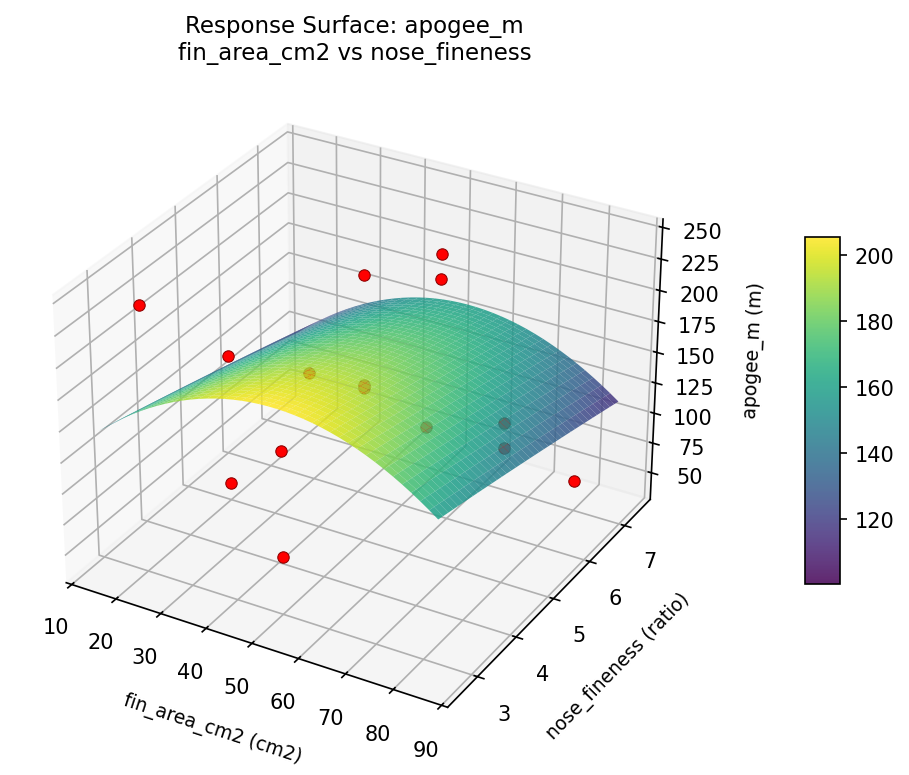
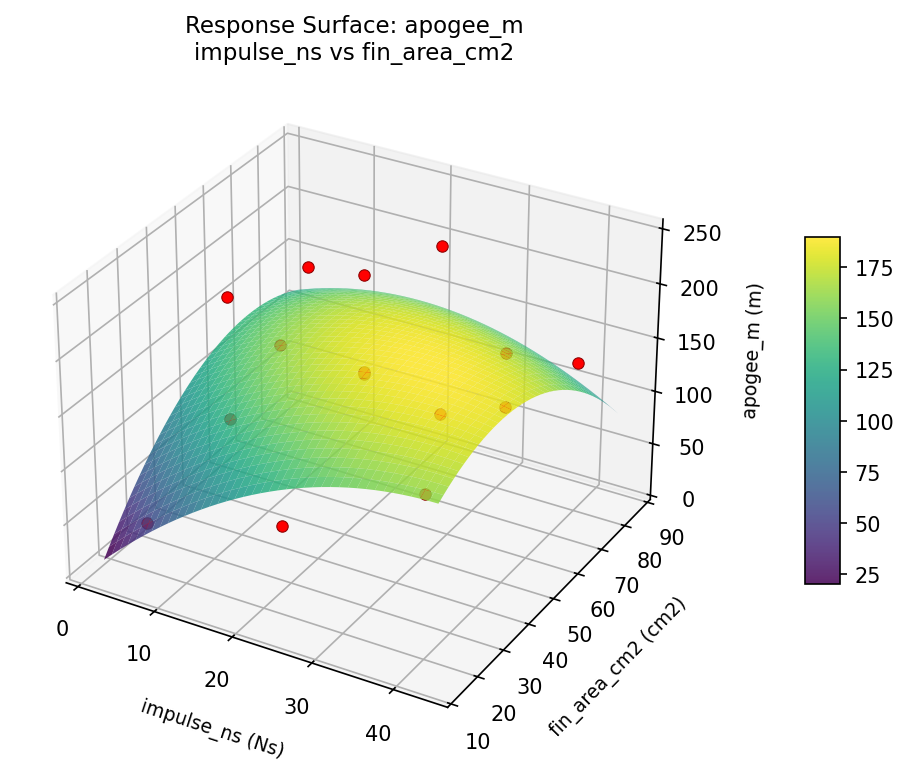
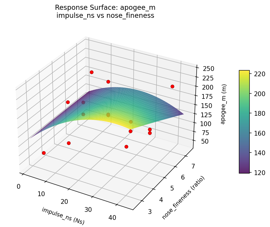
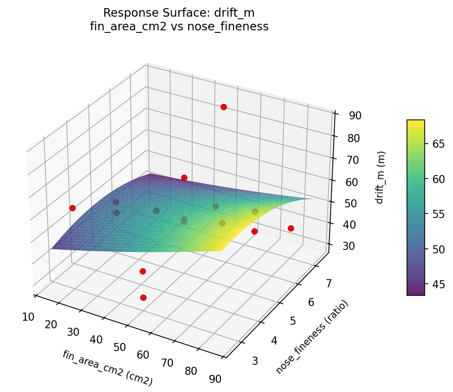
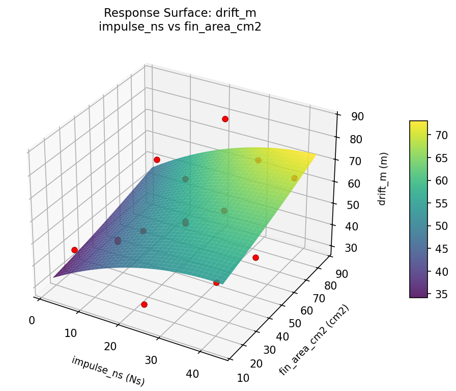
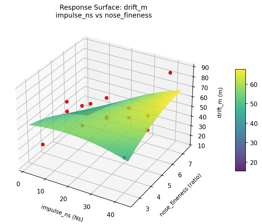
Response Surface Plots
3D surfaces fitted with quadratic RSM. Red dots are observed data points.
apogee m fin area cm2 vs nose fineness
apogee m impulse ns vs fin area cm2
apogee m impulse ns vs nose fineness
drift m fin area cm2 vs nose fineness
drift m impulse ns vs fin area cm2
drift m impulse ns vs nose fineness
Multi-Objective Optimization
When responses compete, Derringer–Suich desirability finds the best compromise.
Each response is scaled to a 0–1 desirability, then combined via a weighted geometric mean.
Overall Desirability
D = 0.8285
Per-Response Desirability
| Response | Weight | Desirability | Predicted | Dir |
|---|
apogee_m |
1.5 |
|
233.45 0.9157 233.45 m |
↑ |
drift_m |
1.0 |
|
45.14 0.7131 45.14 m |
↓ |
Recommended Settings
| Factor | Value |
|---|
impulse_ns | 40 Ns |
fin_area_cm2 | 80 cm2 |
nose_fineness | 5.8 ratio |
Source: from RSM model prediction
Trade-off Summary
Sacrifice = how much worse than single-objective best.
| Response | Predicted | Best Observed | Sacrifice |
|---|
drift_m | 45.14 | 30.00 | +15.14 |
Top 3 Runs by Desirability
| Run | D | Factor Settings |
|---|
| #8 | 0.6907 | impulse_ns=22.5, fin_area_cm2=80, nose_fineness=7 |
| #1 | 0.6345 | impulse_ns=5, fin_area_cm2=80, nose_fineness=5 |
Model Quality
| Response | R² | Type |
|---|
drift_m | 0.9104 | quadratic |
Full Multi-Objective Output
============================================================
MULTI-OBJECTIVE OPTIMIZATION
Method: Derringer-Suich Desirability Function
============================================================
Overall desirability: D = 0.8285
Response Weight Desirability Predicted Direction
---------------------------------------------------------------------
apogee_m 1.5 0.9157 233.45 m ↑
drift_m 1.0 0.7131 45.14 m ↓
Recommended settings:
impulse_ns = 40 Ns
fin_area_cm2 = 80 cm2
nose_fineness = 5.8 ratio
(from RSM model prediction)
Trade-off summary:
apogee_m: 233.45 (best observed: 242.00, sacrifice: +8.55)
drift_m: 45.14 (best observed: 30.00, sacrifice: +15.14)
Model quality:
apogee_m: R² = 0.8841 (quadratic)
drift_m: R² = 0.9104 (quadratic)
Top 3 observed runs by overall desirability:
1. Run #9 (D=0.7824): impulse_ns=40, fin_area_cm2=80, nose_fineness=5
2. Run #8 (D=0.6907): impulse_ns=22.5, fin_area_cm2=80, nose_fineness=7
3. Run #1 (D=0.6345): impulse_ns=5, fin_area_cm2=80, nose_fineness=5
Full Analysis Output
=== Main Effects: apogee_m ===
Factor Effect Std Error % Contribution
--------------------------------------------------------------
impulse_ns 49.0357 16.5584 36.7%
fin_area_cm2 43.4286 16.5584 32.5%
nose_fineness 41.0714 16.5584 30.8%
=== ANOVA Table: apogee_m ===
Source DF SS MS F p-value
-----------------------------------------------------------------------------
impulse_ns 2 6262.4214 3131.2107 8.938 0.0091
fin_area_cm2 2 5931.8857 2965.9429 8.466 0.0106
nose_fineness 2 4338.1357 2169.0679 6.191 0.0237
Lack of Fit 6 40344.4905 6724.0817 19.193 0.0503
Pure Error 2 700.6667 350.3333
Error 8 41045.1571 350.3333
Total 14 57577.6000 4112.6857
=== Summary Statistics: apogee_m ===
impulse_ns:
Level N Mean Std Min Max
------------------------------------------------------------
22.5 7 169.2857 51.0970 79.0000 241.0000
40 4 120.2500 76.4303 42.0000 210.0000
5 4 144.5000 77.7282 52.0000 242.0000
fin_area_cm2:
Level N Mean Std Min Max
------------------------------------------------------------
20 4 172.0000 71.2227 79.0000 242.0000
50 7 128.5714 51.5392 42.0000 188.0000
80 4 164.0000 82.6438 52.0000 241.0000
nose_fineness:
Level N Mean Std Min Max
------------------------------------------------------------
3 4 146.7500 81.5695 42.0000 241.0000
5 7 165.5714 59.9023 52.0000 242.0000
7 4 124.5000 62.5806 74.0000 208.0000
=== Main Effects: drift_m ===
Factor Effect Std Error % Contribution
--------------------------------------------------------------
fin_area_cm2 14.4286 4.4811 76.1%
impulse_ns 4.1429 4.4811 21.8%
nose_fineness 0.3929 4.4811 2.1%
=== ANOVA Table: drift_m ===
Source DF SS MS F p-value
-----------------------------------------------------------------------------
impulse_ns 2 47.3262 23.6631 0.287 0.7576
fin_area_cm2 2 738.4690 369.2345 4.485 0.0494
nose_fineness 2 0.5762 0.2881 0.003 0.9965
Lack of Fit 6 3265.8952 544.3159 6.611 0.1372
Pure Error 2 164.6667 82.3333
Error 8 3430.5619 82.3333
Total 14 4216.9333 301.2095
=== Summary Statistics: drift_m ===
impulse_ns:
Level N Mean Std Min Max
------------------------------------------------------------
22.5 7 51.8571 19.4287 30.0000 87.0000
40 4 52.2500 21.2348 32.0000 82.0000
5 4 56.0000 13.5647 40.0000 70.0000
fin_area_cm2:
Level N Mean Std Min Max
------------------------------------------------------------
20 4 59.2500 22.4109 30.0000 82.0000
50 7 45.5714 11.0583 32.0000 64.0000
80 4 60.0000 20.3142 40.0000 87.0000
nose_fineness:
Level N Mean Std Min Max
------------------------------------------------------------
3 4 53.2500 7.6757 45.0000 63.0000
5 7 52.8571 17.2861 33.0000 82.0000
7 4 53.2500 27.3663 30.0000 87.0000
Optimization Recommendations
=== Optimization: apogee_m ===
Direction: maximize
Best observed run: #3
impulse_ns = 22.5
fin_area_cm2 = 50
nose_fineness = 5
Value: 242.0
RSM Model (linear, R² = 0.3635, Adj R² = 0.1899):
Coefficients:
intercept +149.6000
impulse_ns +19.5000
fin_area_cm2 -7.8750
nose_fineness -46.6250
RSM Model (quadratic, R² = 0.8093, Adj R² = 0.4662):
Coefficients:
intercept +220.0000
impulse_ns +19.5000
fin_area_cm2 -7.8750
nose_fineness -46.6250
impulse_ns*fin_area_cm2 -23.2500
impulse_ns*nose_fineness -15.7500
fin_area_cm2*nose_fineness +3.0000
impulse_ns^2 -69.0000
fin_area_cm2^2 -27.2500
nose_fineness^2 -35.7500
Curvature analysis:
impulse_ns coef=-69.0000 concave (has a maximum)
nose_fineness coef=-35.7500 concave (has a maximum)
fin_area_cm2 coef=-27.2500 concave (has a maximum)
Notable interactions:
impulse_ns*fin_area_cm2 coef=-23.2500 (antagonistic)
impulse_ns*nose_fineness coef=-15.7500 (antagonistic)
fin_area_cm2*nose_fineness coef=+3.0000 (synergistic)
Predicted optimum (from quadratic model, at observed points):
impulse_ns = 22.5
fin_area_cm2 = 50
nose_fineness = 5
Predicted value: 220.0000
Surface optimum (via L-BFGS-B, quadratic model):
impulse_ns = 27.311
fin_area_cm2 = 40.949
nose_fineness = 3.54937
Predicted value: 240.7773
Model quality: Good fit — general trends are captured, some noise remains.
Factor importance:
1. nose_fineness (effect: 93.2, contribution: 45.5%)
2. impulse_ns (effect: 84.0, contribution: 41.0%)
3. fin_area_cm2 (effect: 27.6, contribution: 13.5%)
=== Optimization: drift_m ===
Direction: minimize
Best observed run: #13
impulse_ns = 22.5
fin_area_cm2 = 80
nose_fineness = 7
Value: 30.0
RSM Model (linear, R² = 0.0855, Adj R² = -0.1638):
Coefficients:
intercept +53.0667
impulse_ns -2.3750
fin_area_cm2 -3.2500
nose_fineness -5.3750
RSM Model (quadratic, R² = 0.8984, Adj R² = 0.7155):
Coefficients:
intercept +79.6667
impulse_ns -2.3750
fin_area_cm2 -3.2500
nose_fineness -5.3750
impulse_ns*fin_area_cm2 -7.5000
impulse_ns*nose_fineness +6.2500
fin_area_cm2*nose_fineness -2.0000
impulse_ns^2 -18.7083
fin_area_cm2^2 -8.9583
nose_fineness^2 -22.2083
Curvature analysis:
nose_fineness coef=-22.2083 concave (has a maximum)
impulse_ns coef=-18.7083 concave (has a maximum)
fin_area_cm2 coef=-8.9583 concave (has a maximum)
Notable interactions:
impulse_ns*fin_area_cm2 coef=-7.5000 (antagonistic)
impulse_ns*nose_fineness coef=+6.2500 (synergistic)
fin_area_cm2*nose_fineness coef=-2.0000 (antagonistic)
Predicted optimum (from quadratic model, at observed points):
impulse_ns = 22.5
fin_area_cm2 = 50
nose_fineness = 5
Predicted value: 79.6667
Surface optimum (via L-BFGS-B, quadratic model):
impulse_ns = 40
fin_area_cm2 = 80
nose_fineness = 7
Predicted value: 15.5417
Model quality: Good fit — general trends are captured, some noise remains.
Factor importance:
1. nose_fineness (effect: 25.6, contribution: 47.6%)
2. impulse_ns (effect: 18.9, contribution: 35.1%)
3. fin_area_cm2 (effect: 9.3, contribution: 17.3%)