Summary
This experiment investigates parachute deployment dynamics. Central composite design to maximize opening reliability and minimize opening shock by tuning deployment altitude, reefing ratio, and slider size.
The design varies 3 factors: deploy alt m (m), ranging from 300 to 1500, reefing pct (%), ranging from 0 to 50, and slider pct (%), ranging from 60 to 100. The goal is to optimize 2 responses: reliability pct (%) (maximize) and opening shock g (g) (minimize). Fixed conditions held constant across all runs include canopy = ram_air, load = 90kg.
A Central Composite Design (CCD) was selected to fit a full quadratic response surface model, including curvature and interaction effects. With 3 factors this produces 22 runs including center points and axial (star) points that extend beyond the factorial range.
Quadratic response surface models were fitted to capture potential curvature and factor interactions. The RSM contour plots below visualize how pairs of factors jointly affect each response.
Key Findings
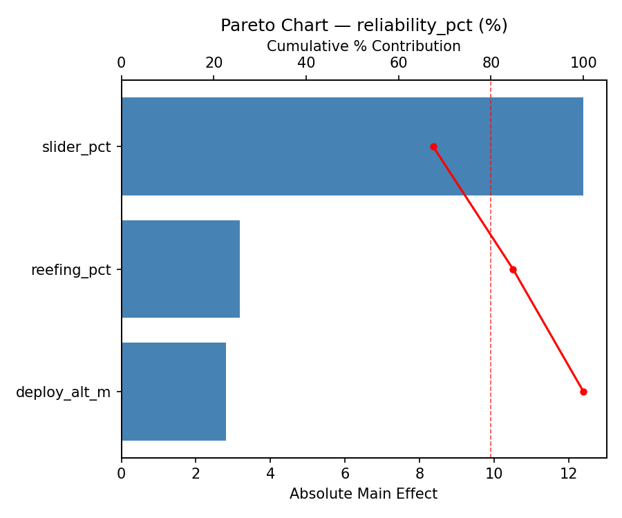
For reliability pct, the most influential factors were reefing pct (57.3%), slider pct (30.2%), deploy alt m (12.5%). The best observed value was 98.7 (at deploy alt m = 1995.45, reefing pct = 25, slider pct = 80).
For opening shock g, the most influential factors were reefing pct (63.4%), deploy alt m (25.4%), slider pct (11.3%). The best observed value was 2.1 (at deploy alt m = 900, reefing pct = 70.6435, slider pct = 80).
Recommended Next Steps
- Run confirmation experiments at the predicted optimal settings to validate the model.
- Consider whether any fixed factors should be varied in a future study.
Experimental Setup
Factors
| Factor | Low | High | Unit |
|---|
deploy_alt_m | 300 | 1500 | m |
reefing_pct | 0 | 50 | % |
slider_pct | 60 | 100 | % |
Fixed: canopy = ram_air, load = 90kg
Responses
| Response | Direction | Unit |
|---|
reliability_pct | ↑ maximize | % |
opening_shock_g | ↓ minimize | g |
Configuration
{
"metadata": {
"name": "Parachute Deployment Dynamics",
"description": "Central composite design to maximize opening reliability and minimize opening shock by tuning deployment altitude, reefing ratio, and slider size"
},
"factors": [
{
"name": "deploy_alt_m",
"levels": [
"300",
"1500"
],
"type": "continuous",
"unit": "m"
},
{
"name": "reefing_pct",
"levels": [
"0",
"50"
],
"type": "continuous",
"unit": "%"
},
{
"name": "slider_pct",
"levels": [
"60",
"100"
],
"type": "continuous",
"unit": "%"
}
],
"fixed_factors": {
"canopy": "ram_air",
"load": "90kg"
},
"responses": [
{
"name": "reliability_pct",
"optimize": "maximize",
"unit": "%"
},
{
"name": "opening_shock_g",
"optimize": "minimize",
"unit": "g"
}
],
"settings": {
"operation": "central_composite",
"test_script": "use_cases/269_parachute_deployment/sim.sh"
}
}
Experimental Matrix
The Central Composite Design produces 22 runs. Each row is one experiment with specific factor settings.
| Run | deploy_alt_m | reefing_pct | slider_pct |
|---|
| 1 | 900 | 25 | 80 |
| 2 | 1500 | 0 | 100 |
| 3 | 300 | 50 | 60 |
| 4 | 900 | 70.6435 | 80 |
| 5 | 900 | 25 | 80 |
| 6 | -195.445 | 25 | 80 |
| 7 | 900 | 25 | 43.4852 |
| 8 | 900 | 25 | 80 |
| 9 | 1500 | 50 | 60 |
| 10 | 1995.45 | 25 | 80 |
| 11 | 900 | 25 | 80 |
| 12 | 900 | -20.6435 | 80 |
| 13 | 900 | 25 | 80 |
| 14 | 300 | 0 | 100 |
| 15 | 900 | 25 | 80 |
| 16 | 1500 | 0 | 60 |
| 17 | 900 | 25 | 116.515 |
| 18 | 1500 | 50 | 100 |
| 19 | 900 | 25 | 80 |
| 20 | 300 | 0 | 60 |
| 21 | 300 | 50 | 100 |
| 22 | 900 | 25 | 80 |
Step-by-Step Workflow
1
Preview the design
$ doe info --config use_cases/269_parachute_deployment/config.json
2
Generate the runner script
$ doe generate --config use_cases/269_parachute_deployment/config.json \
--output use_cases/269_parachute_deployment/results/run.sh --seed 42
3
Execute the experiments
$ bash use_cases/269_parachute_deployment/results/run.sh
4
Analyze results
$ doe analyze --config use_cases/269_parachute_deployment/config.json
5
Get optimization recommendations
$ doe optimize --config use_cases/269_parachute_deployment/config.json
6
Multi-objective optimization
With 2 competing responses, use --multi to find the best compromise via Derringer–Suich desirability.
$ doe optimize --config use_cases/269_parachute_deployment/config.json --multi
7
Generate the HTML report
$ doe report --config use_cases/269_parachute_deployment/config.json \
--output use_cases/269_parachute_deployment/results/report.html
Features Exercised
| Feature | Value |
|---|
| Design type | central_composite |
| Factor types | continuous (all 3) |
| Arg style | double-dash |
| Responses | 2 (reliability_pct ↑, opening_shock_g ↓) |
| Total runs | 22 |
Analysis Results
Generated from actual experiment runs using the DOE Helper Tool.
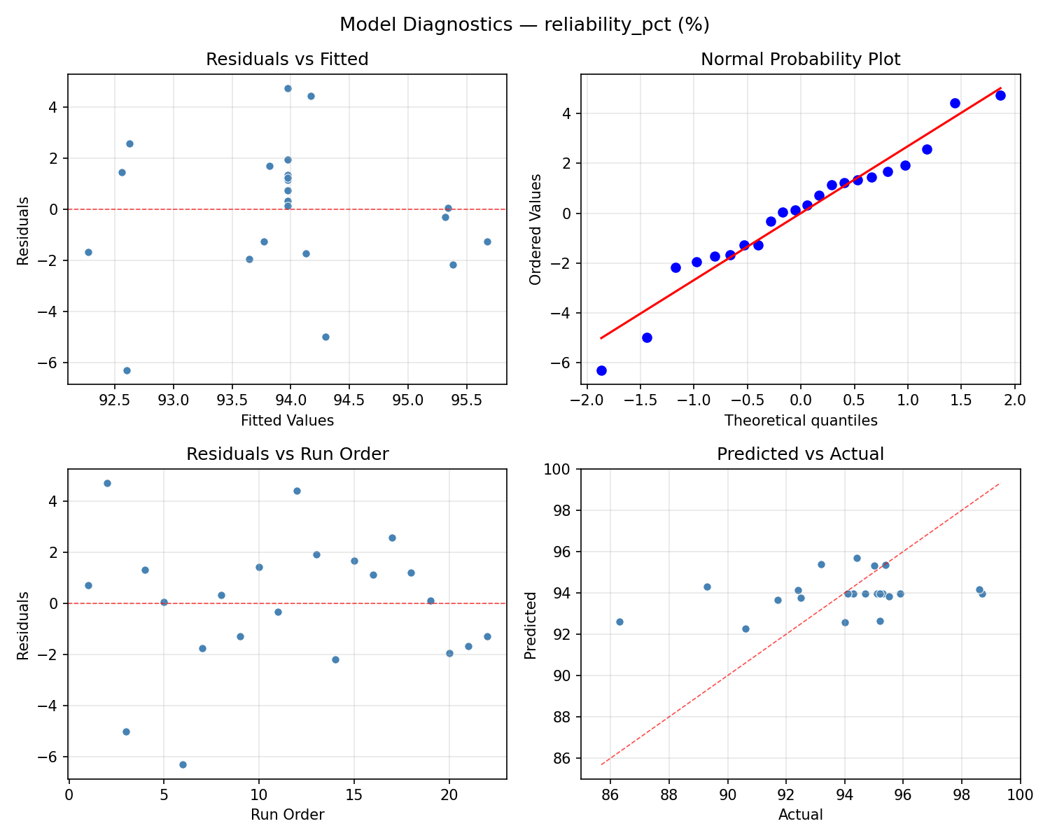
Response: reliability_pct
Top factors: reefing_pct (57.3%), slider_pct (30.2%), deploy_alt_m (12.5%).
ANOVA
| Source | DF | SS | MS | F | p-value |
|---|
| Source | DF | SS | MS | F | p-value |
| deploy_alt_m | 4 | 7.4895 | 1.8724 | 0.217 | 0.9226 |
| reefing_pct | 4 | 29.6870 | 7.4217 | 0.859 | 0.5238 |
| slider_pct | 4 | 16.9270 | 4.2317 | 0.490 | 0.7440 |
| Lack | of | Fit | 2 | 47.6452 | 23.8226 |
| Pure | Error | 7 | 60.5150 | | |
| Error | 9 | 108.1602 | 8.6450 | | |
| Total | 21 | 162.2636 | 7.7268 | | |
Pareto Chart
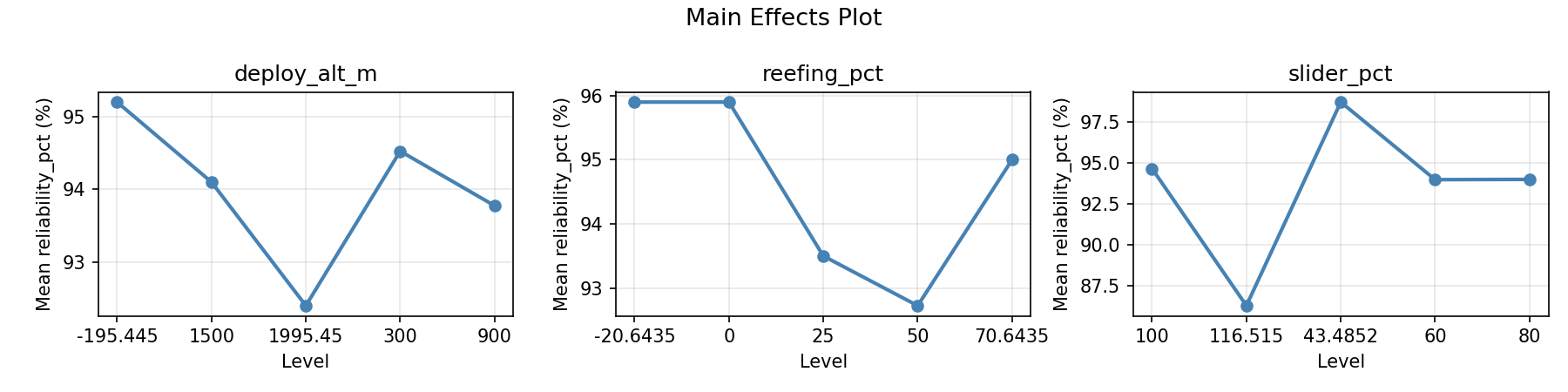
Main Effects Plot
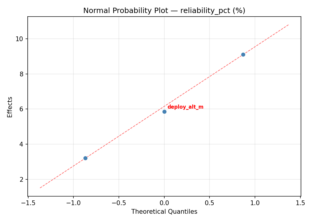
Normal Probability Plot of Effects
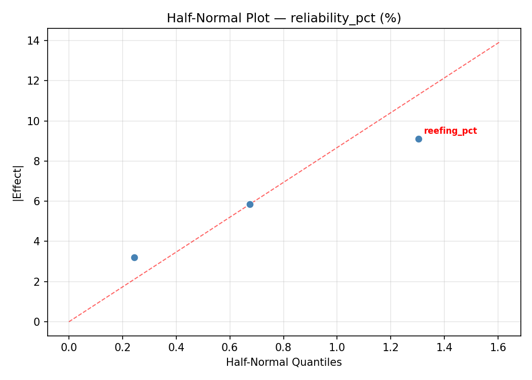
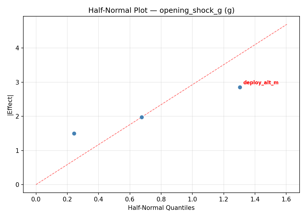
Half-Normal Plot of Effects
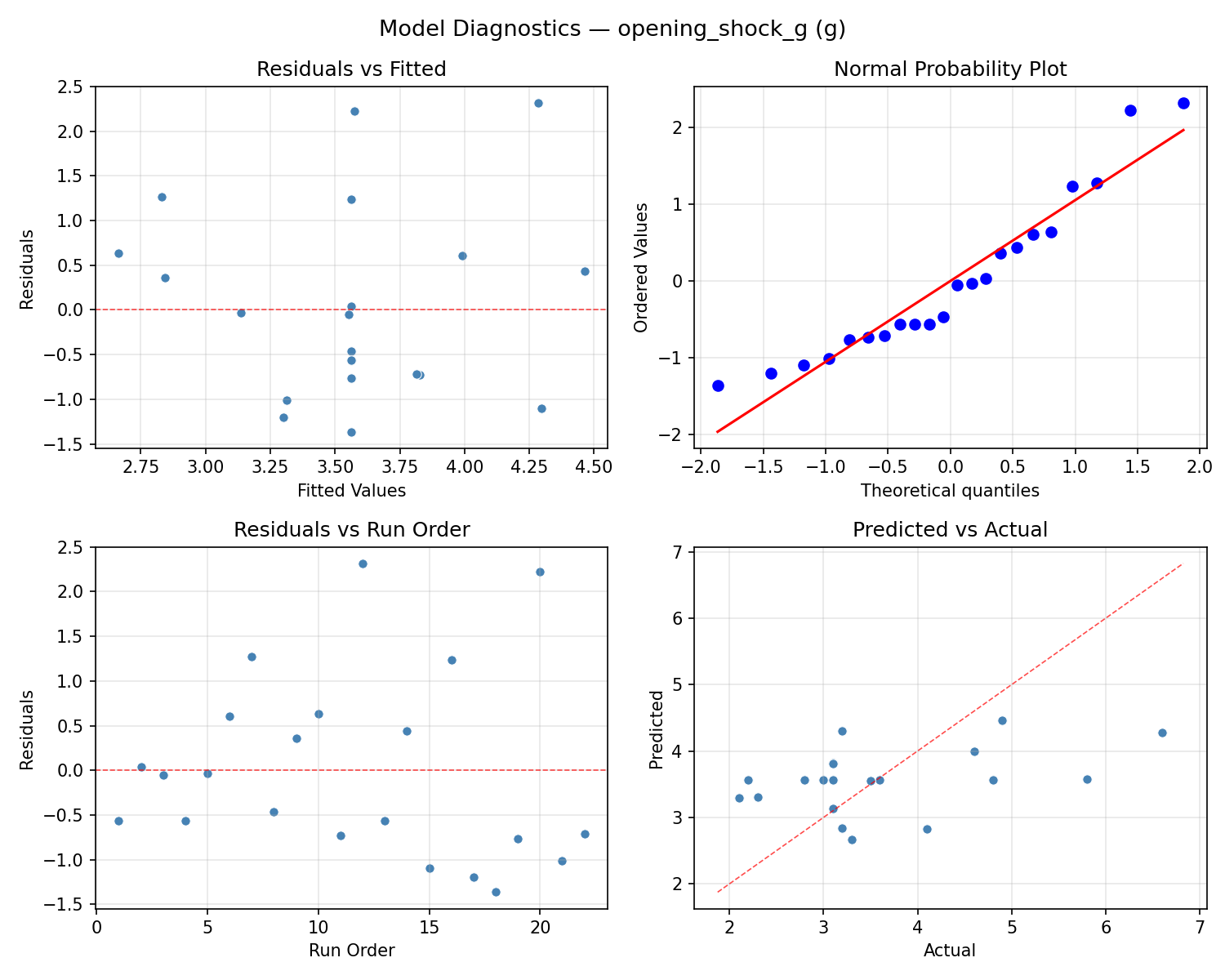
Model Diagnostics
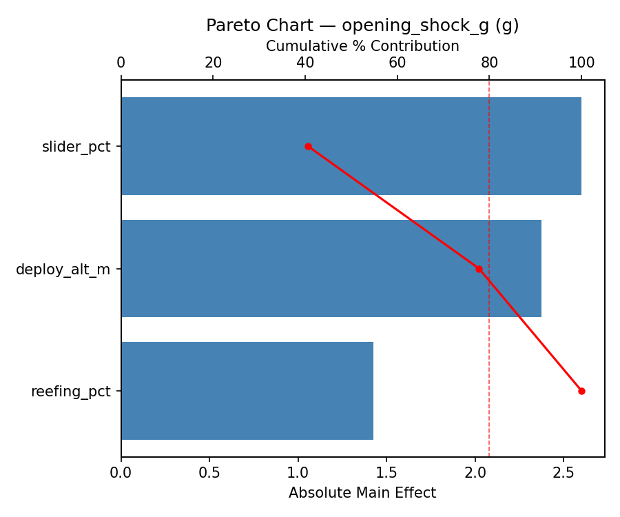
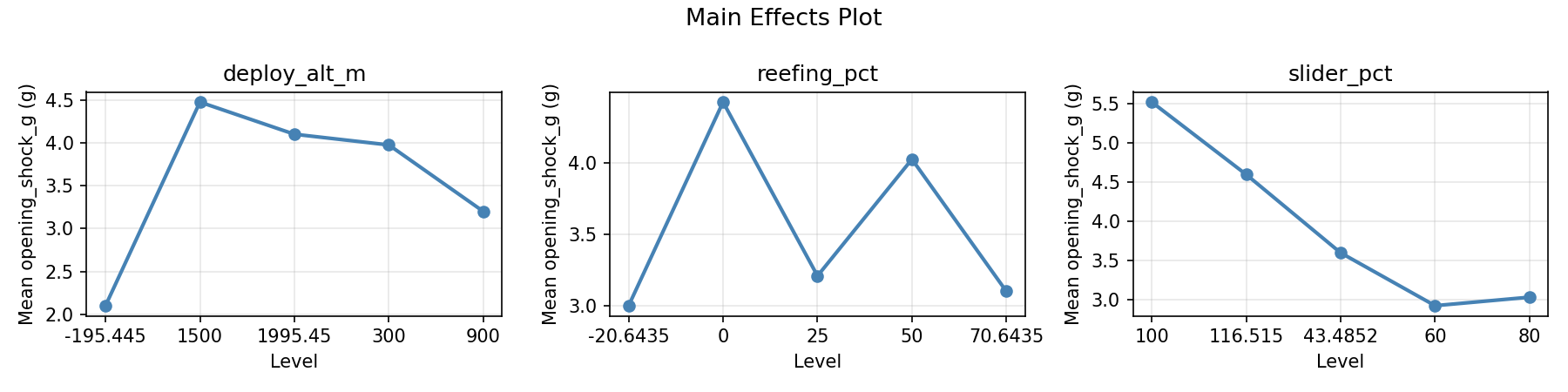
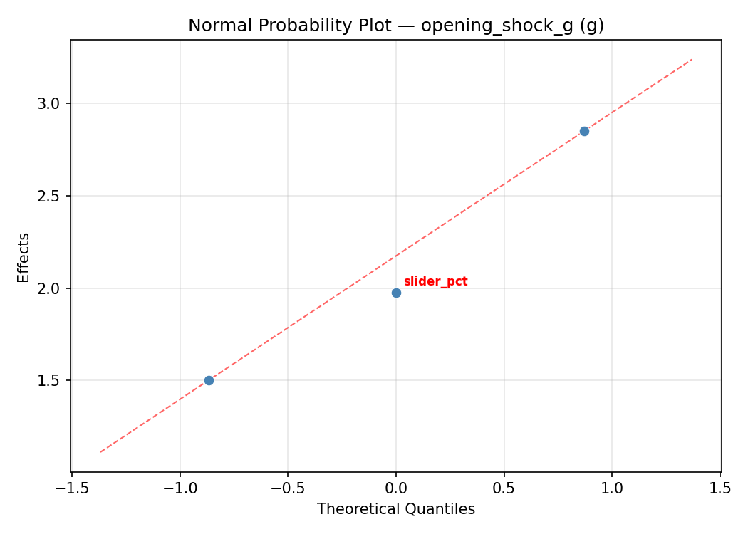
Response: opening_shock_g
Top factors: reefing_pct (63.4%), deploy_alt_m (25.4%), slider_pct (11.3%).
ANOVA
| Source | DF | SS | MS | F | p-value |
|---|
| Source | DF | SS | MS | F | p-value |
| deploy_alt_m | 4 | 2.5909 | 0.6477 | 0.821 | 0.5431 |
| reefing_pct | 4 | 12.0567 | 3.0142 | 3.822 | 0.0440 |
| slider_pct | 4 | 0.8742 | 0.2186 | 0.277 | 0.8855 |
| Lack | of | Fit | 2 | 6.1890 | 3.0945 |
| Pure | Error | 7 | 5.5200 | | |
| Error | 9 | 11.7090 | 0.7886 | | |
| Total | 21 | 27.2309 | 1.2967 | | |
Pareto Chart
Main Effects Plot
Normal Probability Plot of Effects
Half-Normal Plot of Effects
Model Diagnostics
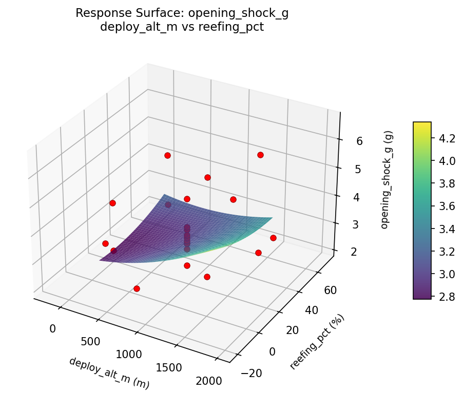
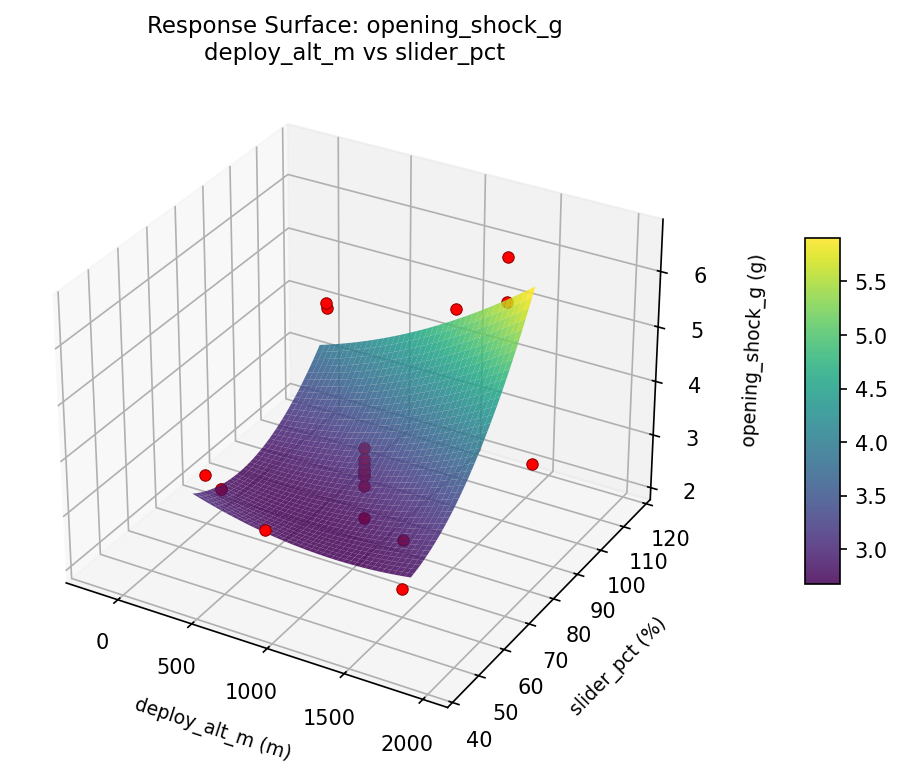
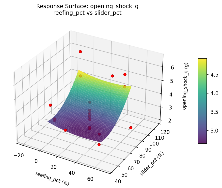
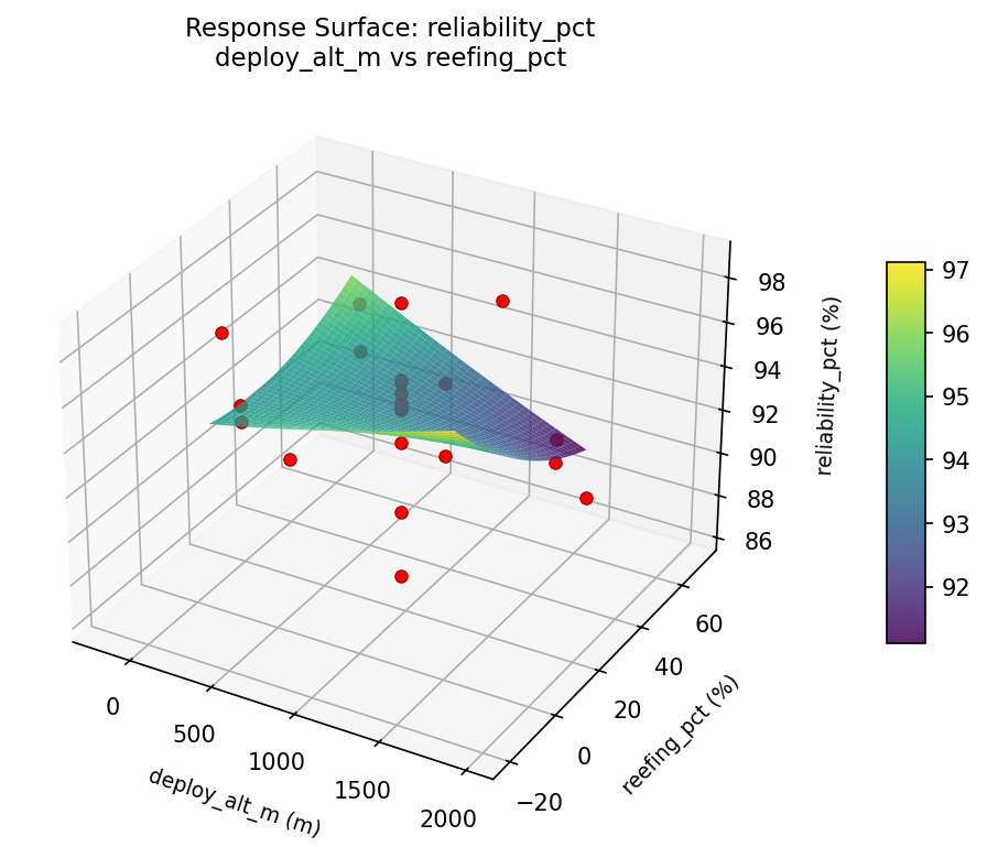
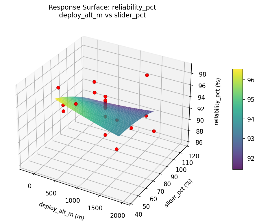
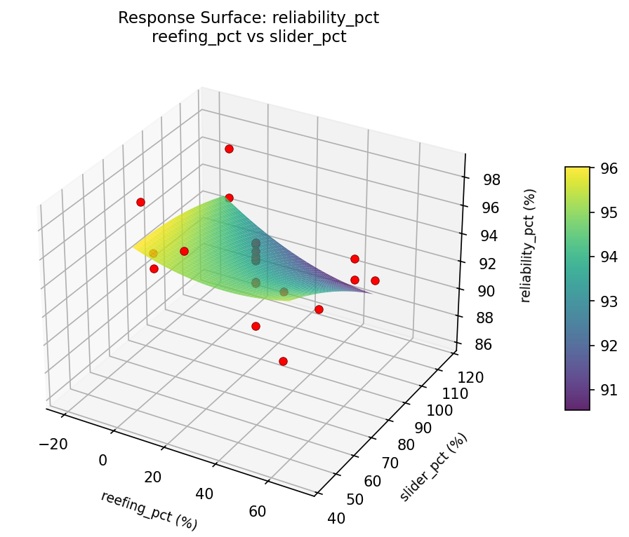
Response Surface Plots
3D surfaces fitted with quadratic RSM. Red dots are observed data points.
opening shock g deploy alt m vs reefing pct
opening shock g deploy alt m vs slider pct
opening shock g reefing pct vs slider pct
reliability pct deploy alt m vs reefing pct
reliability pct deploy alt m vs slider pct
reliability pct reefing pct vs slider pct
Multi-Objective Optimization
When responses compete, Derringer–Suich desirability finds the best compromise.
Each response is scaled to a 0–1 desirability, then combined via a weighted geometric mean.
Overall Desirability
D = 0.8307
Per-Response Desirability
| Response | Weight | Desirability | Predicted | Dir |
|---|
reliability_pct |
1.5 |
|
97.53 0.8685 97.53 % |
↑ |
opening_shock_g |
1.0 |
|
2.98 0.7771 2.98 g |
↓ |
Recommended Settings
| Factor | Value |
|---|
deploy_alt_m | 1500 m |
reefing_pct | 0 % |
slider_pct | 100 % |
Source: from RSM model prediction
Trade-off Summary
Sacrifice = how much worse than single-objective best.
| Response | Predicted | Best Observed | Sacrifice |
|---|
opening_shock_g | 2.98 | 2.10 | +0.88 |
Top 3 Runs by Desirability
| Run | D | Factor Settings |
|---|
| #17 | 0.7911 | deploy_alt_m=900, reefing_pct=70.6435, slider_pct=80 |
| #18 | 0.7843 | deploy_alt_m=-195.445, reefing_pct=25, slider_pct=80 |
Model Quality
| Response | R² | Type |
|---|
opening_shock_g | 0.5424 | quadratic |
Full Multi-Objective Output
============================================================
MULTI-OBJECTIVE OPTIMIZATION
Method: Derringer-Suich Desirability Function
============================================================
Overall desirability: D = 0.8307
Response Weight Desirability Predicted Direction
---------------------------------------------------------------------
reliability_pct 1.5 0.8685 97.53 % ↑
opening_shock_g 1.0 0.7771 2.98 g ↓
Recommended settings:
deploy_alt_m = 1500 m
reefing_pct = 0 %
slider_pct = 100 %
(from RSM model prediction)
Trade-off summary:
reliability_pct: 97.53 (best observed: 98.70, sacrifice: +1.17)
opening_shock_g: 2.98 (best observed: 2.10, sacrifice: +0.88)
Model quality:
reliability_pct: R² = 0.3567 (quadratic)
opening_shock_g: R² = 0.5424 (quadratic)
Top 3 observed runs by overall desirability:
1. Run #2 (D=0.8193): deploy_alt_m=1500, reefing_pct=0, slider_pct=100
2. Run #17 (D=0.7911): deploy_alt_m=900, reefing_pct=70.6435, slider_pct=80
3. Run #18 (D=0.7843): deploy_alt_m=-195.445, reefing_pct=25, slider_pct=80
Full Analysis Output
=== Main Effects: reliability_pct ===
Factor Effect Std Error % Contribution
--------------------------------------------------------------
reefing_pct 5.9250 0.5926 57.3%
slider_pct 3.1250 0.5926 30.2%
deploy_alt_m 1.2917 0.5926 12.5%
=== ANOVA Table: reliability_pct ===
Source DF SS MS F p-value
-----------------------------------------------------------------------------
deploy_alt_m 4 7.4895 1.8724 0.217 0.9226
reefing_pct 4 29.6870 7.4217 0.859 0.5238
slider_pct 4 16.9270 4.2317 0.490 0.7440
Lack of Fit 2 47.6452 23.8226 2.756 0.1310
Pure Error 7 60.5150 8.6450
Error 9 108.1602 8.6450
Total 21 162.2636 7.7268
=== Summary Statistics: reliability_pct ===
deploy_alt_m:
Level N Mean Std Min Max
------------------------------------------------------------
-195.445 1 94.3000 0.0000 94.3000 94.3000
1500 4 93.4000 1.6391 91.7000 95.4000
1995.45 1 93.2000 0.0000 93.2000 93.2000
300 4 93.1750 4.5981 86.3000 95.9000
900 12 94.4667 2.7516 89.3000 98.7000
reefing_pct:
Level N Mean Std Min Max
------------------------------------------------------------
-20.6435 1 95.2000 0.0000 95.2000 95.2000
0 4 92.6750 4.2906 86.3000 95.4000
25 12 93.9417 2.4119 89.3000 98.7000
50 4 93.9000 2.1103 91.7000 95.9000
70.6435 1 98.6000 0.0000 98.6000 98.6000
slider_pct:
Level N Mean Std Min Max
------------------------------------------------------------
100 4 92.1750 4.1564 86.3000 95.9000
116.515 1 95.3000 0.0000 95.3000 95.3000
43.4852 1 94.7000 0.0000 94.7000 94.7000
60 4 94.4000 1.8129 91.7000 95.5000
80 12 94.2583 2.7576 89.3000 98.7000
=== Main Effects: opening_shock_g ===
Factor Effect Std Error % Contribution
--------------------------------------------------------------
reefing_pct 4.5000 0.2428 63.4%
deploy_alt_m 1.8000 0.2428 25.4%
slider_pct 0.8000 0.2428 11.3%
=== ANOVA Table: opening_shock_g ===
Source DF SS MS F p-value
-----------------------------------------------------------------------------
deploy_alt_m 4 2.5909 0.6477 0.821 0.5431
reefing_pct 4 12.0567 3.0142 3.822 0.0440
slider_pct 4 0.8742 0.2186 0.277 0.8855
Lack of Fit 2 6.1890 3.0945 3.924 0.0719
Pure Error 7 5.5200 0.7886
Error 9 11.7090 0.7886
Total 21 27.2309 1.2967
=== Summary Statistics: opening_shock_g ===
deploy_alt_m:
Level N Mean Std Min Max
------------------------------------------------------------
-195.445 1 3.1000 0.0000 3.1000 3.1000
1500 4 3.8500 1.3026 3.1000 5.8000
1995.45 1 4.9000 0.0000 4.9000 4.9000
300 4 3.4750 0.7544 3.0000 4.6000
900 12 3.4250 1.2736 2.1000 6.6000
reefing_pct:
Level N Mean Std Min Max
------------------------------------------------------------
-20.6435 1 2.1000 0.0000 2.1000 2.1000
0 4 3.5250 0.7228 3.1000 4.6000
25 12 3.3667 0.8659 2.2000 4.9000
50 4 3.8000 1.3367 3.0000 5.8000
70.6435 1 6.6000 0.0000 6.6000 6.6000
slider_pct:
Level N Mean Std Min Max
------------------------------------------------------------
100 4 3.5250 0.7274 3.0000 4.6000
116.515 1 3.0000 0.0000 3.0000 3.0000
43.4852 1 3.0000 0.0000 3.0000 3.0000
60 4 3.8000 1.3342 3.1000 5.8000
80 12 3.5917 1.3290 2.1000 6.6000
Optimization Recommendations
=== Optimization: reliability_pct ===
Direction: maximize
Best observed run: #2
deploy_alt_m = 1995.45
reefing_pct = 25
slider_pct = 80
Value: 98.7
RSM Model (linear, R² = 0.0504, Adj R² = -0.1079):
Coefficients:
intercept +93.9727
deploy_alt_m +0.3957
reefing_pct -0.0258
slider_pct +0.6328
RSM Model (quadratic, R² = 0.2548, Adj R² = -0.3042):
Coefficients:
intercept +92.8583
deploy_alt_m +0.3957
reefing_pct -0.0258
slider_pct +0.6328
deploy_alt_m*reefing_pct +0.1875
deploy_alt_m*slider_pct -0.1875
reefing_pct*slider_pct +0.5125
deploy_alt_m^2 +1.0472
reefing_pct^2 +0.7022
slider_pct^2 -0.0778
Curvature analysis:
deploy_alt_m coef=+1.0472 convex (has a minimum)
reefing_pct coef=+0.7022 convex (has a minimum)
slider_pct coef=-0.0778 negligible curvature
Notable interactions:
reefing_pct*slider_pct coef=+0.5125 (synergistic)
Predicted optimum (from linear model, at observed points):
deploy_alt_m = 900
reefing_pct = 25
slider_pct = 116.515
Predicted value: 95.1281
Surface optimum (via L-BFGS-B, linear model):
deploy_alt_m = 1500
reefing_pct = 0
slider_pct = 100
Predicted value: 95.0270
Model quality: Weak fit — consider adding center points or using a different design.
Factor importance:
1. deploy_alt_m (effect: 5.4, contribution: 43.1%)
2. slider_pct (effect: 4.7, contribution: 37.8%)
3. reefing_pct (effect: 2.4, contribution: 19.0%)
=== Optimization: opening_shock_g ===
Direction: minimize
Best observed run: #17
deploy_alt_m = 900
reefing_pct = 70.6435
slider_pct = 80
Value: 2.1
RSM Model (linear, R² = 0.0975, Adj R² = -0.0529):
Coefficients:
intercept +3.5636
deploy_alt_m +0.3747
reefing_pct -0.1802
slider_pct -0.0901
RSM Model (quadratic, R² = 0.2417, Adj R² = -0.3269):
Coefficients:
intercept +4.0110
deploy_alt_m +0.3747
reefing_pct -0.1802
slider_pct -0.0901
deploy_alt_m*reefing_pct -0.0750
deploy_alt_m*slider_pct -0.2750
reefing_pct*slider_pct -0.1000
deploy_alt_m^2 -0.0837
reefing_pct^2 -0.3087
slider_pct^2 -0.2787
Curvature analysis:
reefing_pct coef=-0.3087 concave (has a maximum)
slider_pct coef=-0.2787 concave (has a maximum)
deploy_alt_m coef=-0.0837 negligible curvature
Predicted optimum (from linear model, at observed points):
deploy_alt_m = 1995.45
reefing_pct = 25
slider_pct = 80
Predicted value: 4.2477
Surface optimum (via L-BFGS-B, linear model):
deploy_alt_m = 300
reefing_pct = 50
slider_pct = 100
Predicted value: 2.9186
Model quality: Weak fit — consider adding center points or using a different design.
Factor importance:
1. slider_pct (effect: 1.7, contribution: 36.7%)
2. reefing_pct (effect: 1.7, contribution: 36.7%)
3. deploy_alt_m (effect: 1.2, contribution: 26.6%)