LED Strip Installation — DOE Use Case

Summary

This experiment investigates led strip installation. Box-Behnken design to maximize brightness uniformity and minimize hot spots by tuning strip density, power supply headroom, and diffuser distance.

The design varies 3 factors: leds per m (LEDs/m), ranging from 30 to 120, psu headroom pct (%), ranging from 10 to 40, and diffuser mm (mm), ranging from 5 to 30. The goal is to optimize 2 responses: uniformity pct (%) (maximize) and hotspot temp c (C) (minimize). Fixed conditions held constant across all runs include voltage = 12V, color = warm_white.

A Box-Behnken design was chosen because it efficiently fits quadratic models with 3 continuous factors while avoiding extreme corner combinations — requiring only 15 runs instead of the 8 needed for a full factorial at two levels.

Quadratic response surface models were fitted to capture potential curvature and factor interactions. The RSM contour plots below visualize how pairs of factors jointly affect each response.

Key Findings

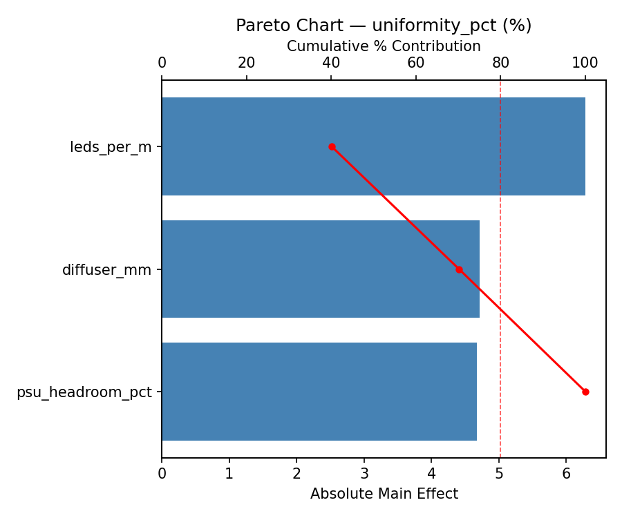
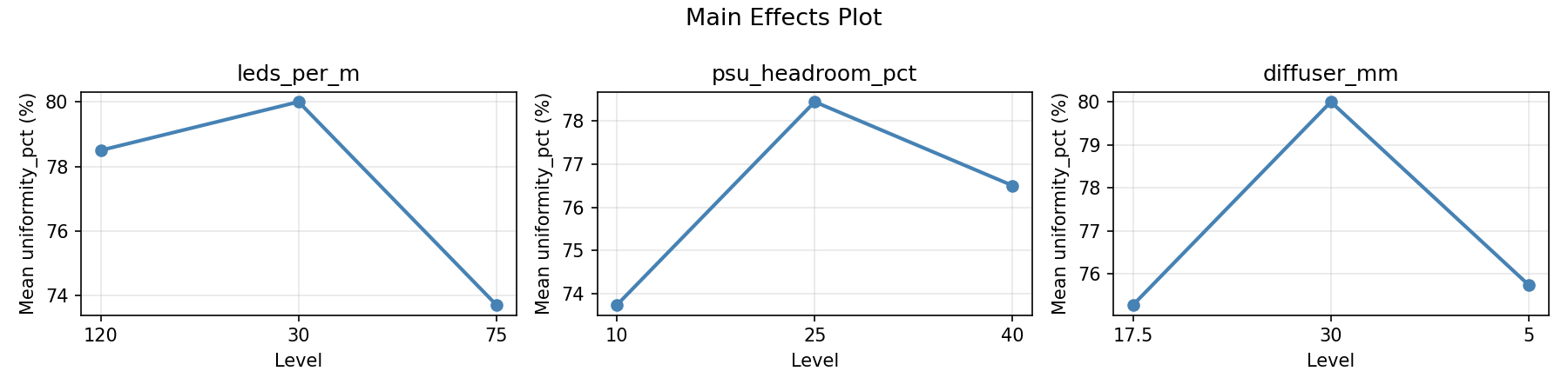
For uniformity pct, the most influential factors were leds per m (75.2%), psu headroom pct (15.7%), diffuser mm (9.1%). The best observed value was 88.0 (at leds per m = 120, psu headroom pct = 25, diffuser mm = 30).

For hotspot temp c, the most influential factors were psu headroom pct (38.0%), diffuser mm (34.2%), leds per m (27.7%). The best observed value was 24.0 (at leds per m = 30, psu headroom pct = 40, diffuser mm = 17.5).

Recommended Next Steps

Run confirmation experiments at the predicted optimal settings to validate the model.
Consider whether any fixed factors should be varied in a future study.

Experimental Setup

Factors

Factor	Low	High	Unit
`leds_per_m`	30	120	LEDs/m
`psu_headroom_pct`	10	40	%
`diffuser_mm`	5	30	mm

Fixed: voltage = 12V, color = warm_white

Responses

Response	Direction	Unit
`uniformity_pct`	↑ maximize	%
`hotspot_temp_c`	↓ minimize	C

Configuration

use_cases/271_led_strip_install/config.json

{
  "metadata": {
    "name": "LED Strip Installation",
    "description": "Box-Behnken design to maximize brightness uniformity and minimize hot spots by tuning strip density, power supply headroom, and diffuser distance"
  },
  "factors": [
    {
      "name": "leds_per_m",
      "levels": [
        "30",
        "120"
      ],
      "type": "continuous",
      "unit": "LEDs/m"
    },
    {
      "name": "psu_headroom_pct",
      "levels": [
        "10",
        "40"
      ],
      "type": "continuous",
      "unit": "%"
    },
    {
      "name": "diffuser_mm",
      "levels": [
        "5",
        "30"
      ],
      "type": "continuous",
      "unit": "mm"
    }
  ],
  "fixed_factors": {
    "voltage": "12V",
    "color": "warm_white"
  },
  "responses": [
    {
      "name": "uniformity_pct",
      "optimize": "maximize",
      "unit": "%"
    },
    {
      "name": "hotspot_temp_c",
      "optimize": "minimize",
      "unit": "C"
    }
  ],
  "settings": {
    "operation": "box_behnken",
    "test_script": "use_cases/271_led_strip_install/sim.sh"
  }
}

Experimental Matrix

The Box-Behnken Design produces 15 runs. Each row is one experiment with specific factor settings.

Run	`leds_per_m`	`psu_headroom_pct`	`diffuser_mm`
1	75	10	5
2	75	25	17.5
3	120	25	30
4	120	25	5
5	75	25	17.5
6	75	25	17.5
7	30	25	30
8	120	10	17.5
9	75	10	30
10	120	40	17.5
11	30	25	5
12	75	40	30
13	30	10	17.5
14	30	40	17.5
15	75	40	5

Step-by-Step Workflow

1

Preview the design

Terminal

$ doe info --config use_cases/271_led_strip_install/config.json

2

Generate the runner script

Terminal

$ doe generate --config use_cases/271_led_strip_install/config.json \
    --output use_cases/271_led_strip_install/results/run.sh --seed 42

3

Execute the experiments

Terminal

$ bash use_cases/271_led_strip_install/results/run.sh

4

Analyze results

Terminal

$ doe analyze --config use_cases/271_led_strip_install/config.json

5

Get optimization recommendations

Terminal

$ doe optimize --config use_cases/271_led_strip_install/config.json

6

Multi-objective optimization

With 2 competing responses, use --multi to find the best compromise via Derringer–Suich desirability.

Terminal

$ doe optimize --config use_cases/271_led_strip_install/config.json --multi

7

Generate the HTML report

Terminal

$ doe report --config use_cases/271_led_strip_install/config.json \
    --output use_cases/271_led_strip_install/results/report.html

Features Exercised

Feature	Value
Design type	`box_behnken`
Factor types	`continuous` (all 3)
Arg style	`double-dash`
Responses	2 (uniformity_pct ↑, hotspot_temp_c ↓)
Total runs	15

Analysis Results

Generated from actual experiment runs using the DOE Helper Tool.

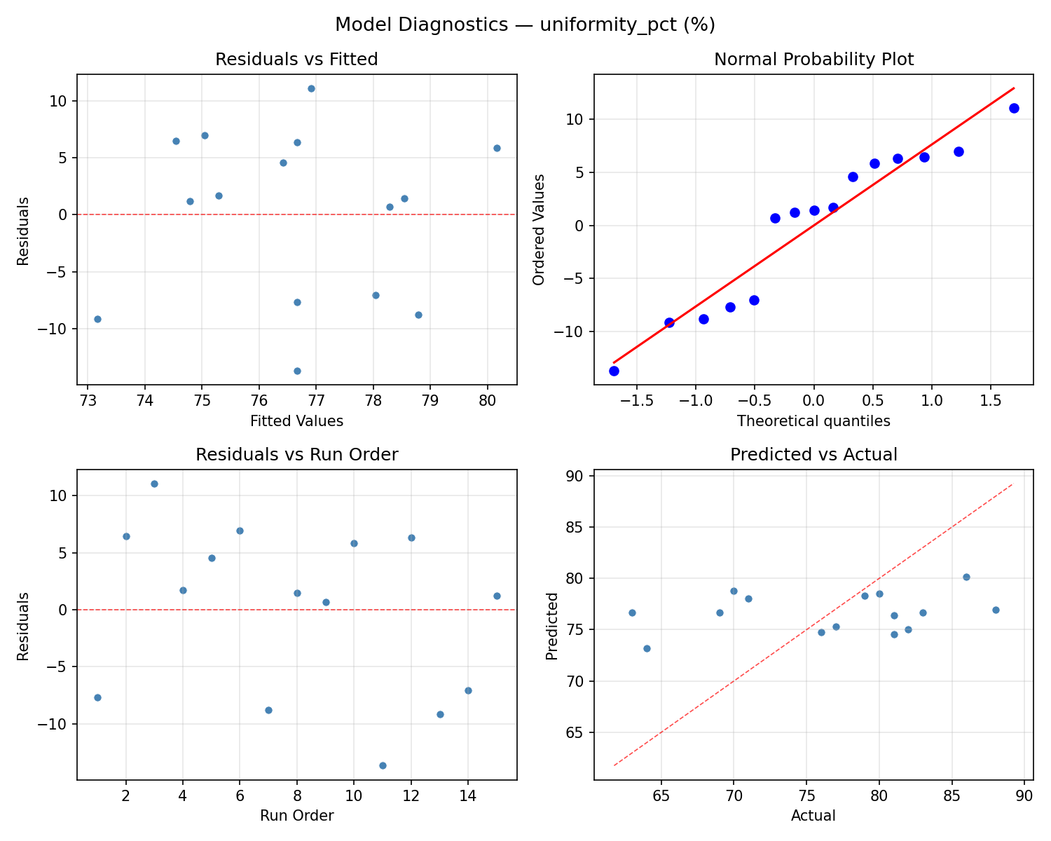
Response: uniformity_pct

Top factors: leds_per_m (75.2%), psu_headroom_pct (15.7%), diffuser_mm (9.1%).

ANOVA

Source	DF	SS	MS	F	p-value
Source	DF	SS	MS	F	p-value
leds_per_m	2	392.4762	196.2381	7.452	0.0149
psu_headroom_pct	2	20.6190	10.3095	0.392	0.6883
diffuser_mm	2	4.9762	2.4881	0.094	0.9108
Lack	of	Fit	6	350.5952	58.4325
Pure	Error	2	52.6667
Error	8	403.2619	26.3333
Total	14	821.3333	58.6667

Pareto Chart

Main Effects Plot

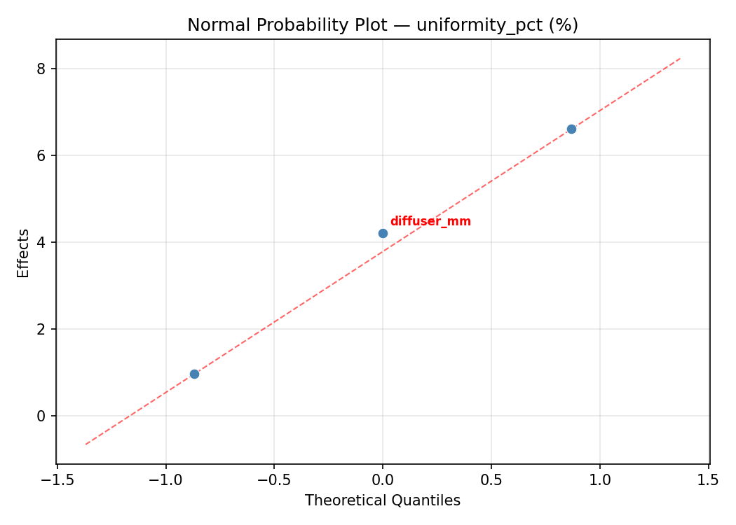
Normal Probability Plot of Effects

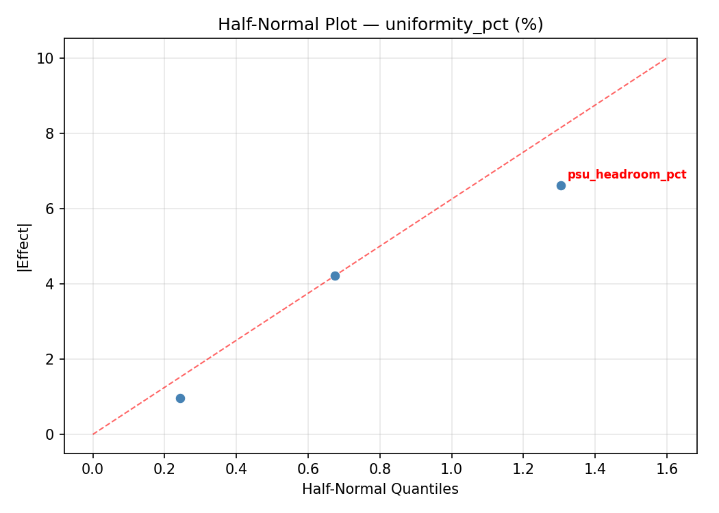
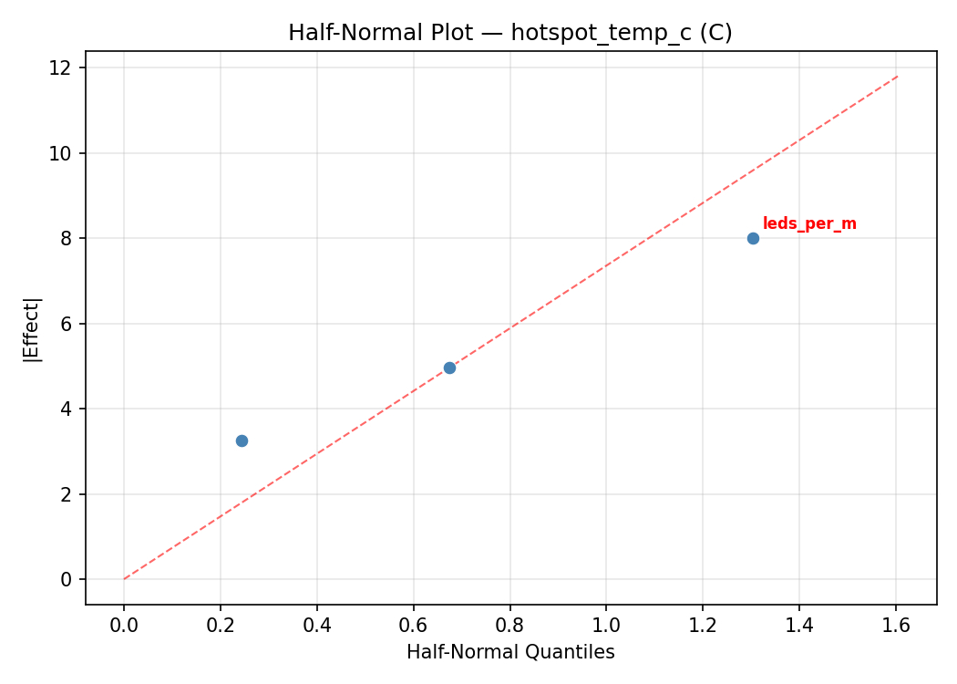
Normal probability plot for uniformity_pct

Half-Normal Plot of Effects

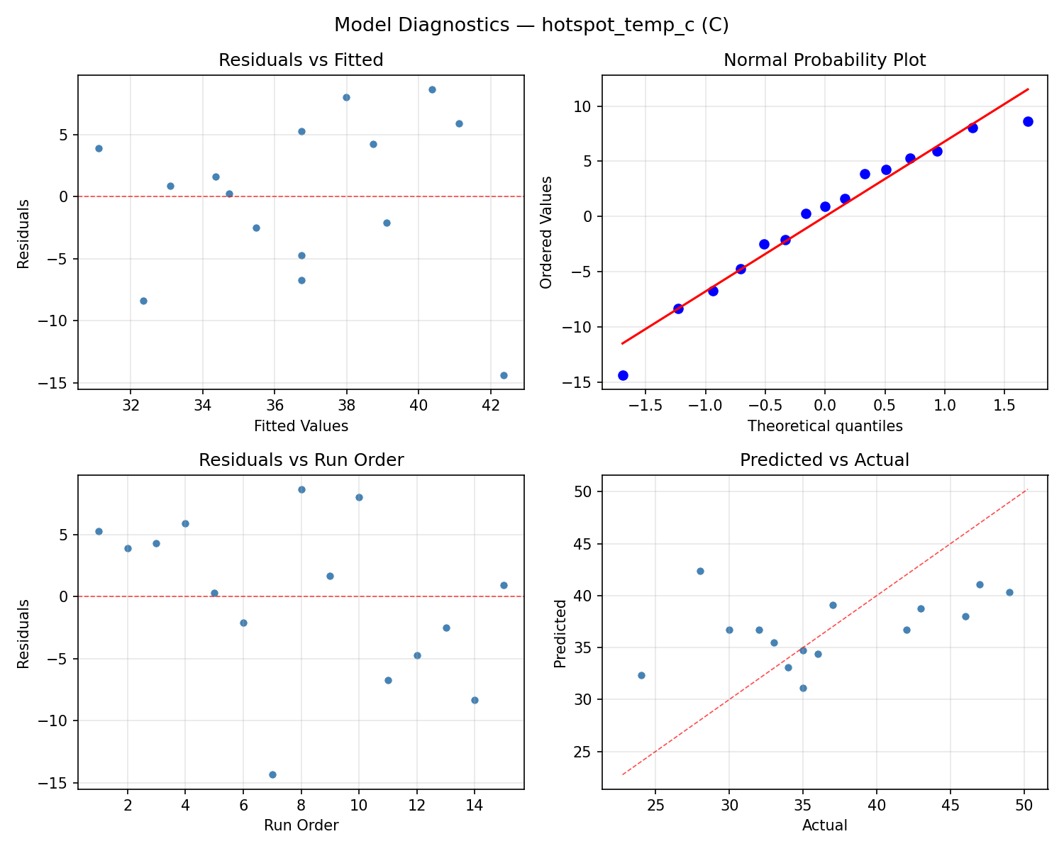
Model Diagnostics

Response: hotspot_temp_c

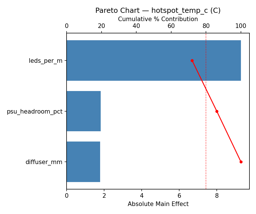
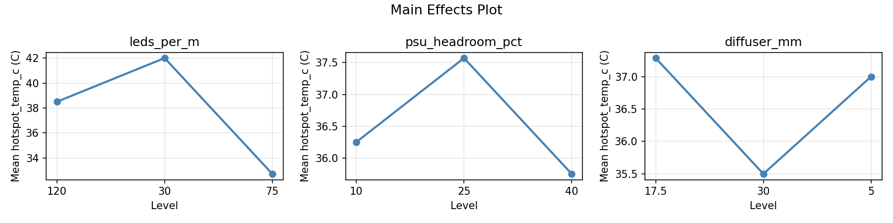
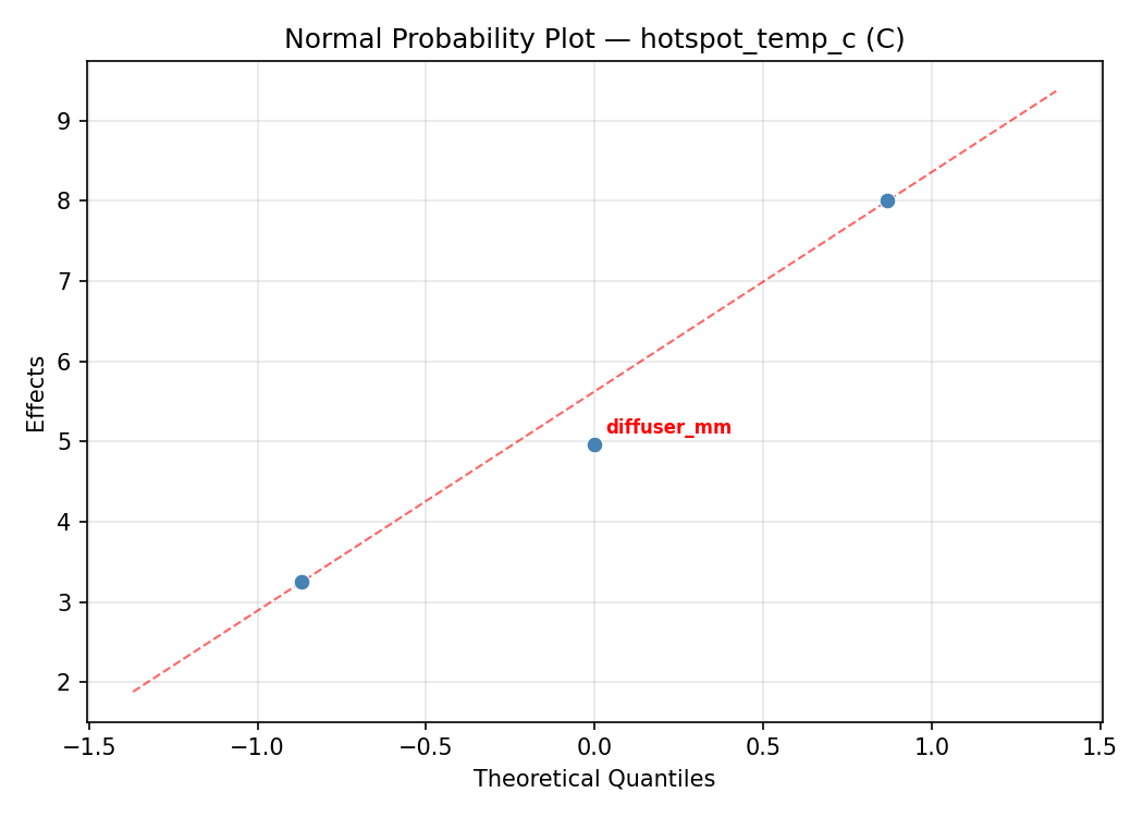
Top factors: psu_headroom_pct (38.0%), diffuser_mm (34.2%), leds_per_m (27.7%).

ANOVA

Source	DF	SS	MS	F	p-value
Source	DF	SS	MS	F	p-value
leds_per_m	2	34.0762	17.0381	0.412	0.6755
psu_headroom_pct	2	50.0048	25.0024	0.605	0.5693
diffuser_mm	2	41.4333	20.7167	0.501	0.6236
Lack	of	Fit	6	534.7524	89.1254
Pure	Error	2	82.6667
Error	8	617.4190	41.3333
Total	14	742.9333	53.0667

Pareto Chart

Main Effects Plot

Normal Probability Plot of Effects

Normal probability plot for hotspot_temp_c

Half-Normal Plot of Effects

Model Diagnostics

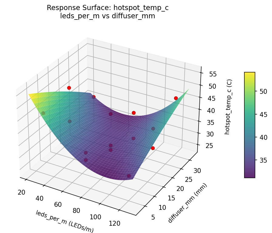
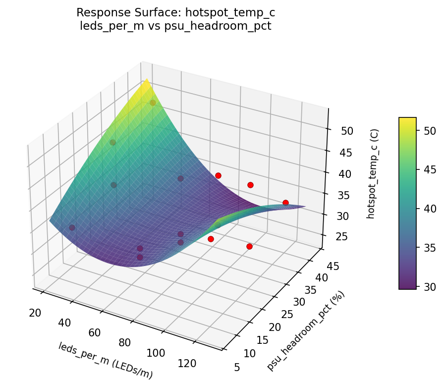
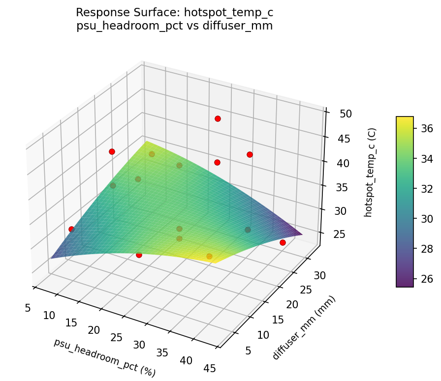
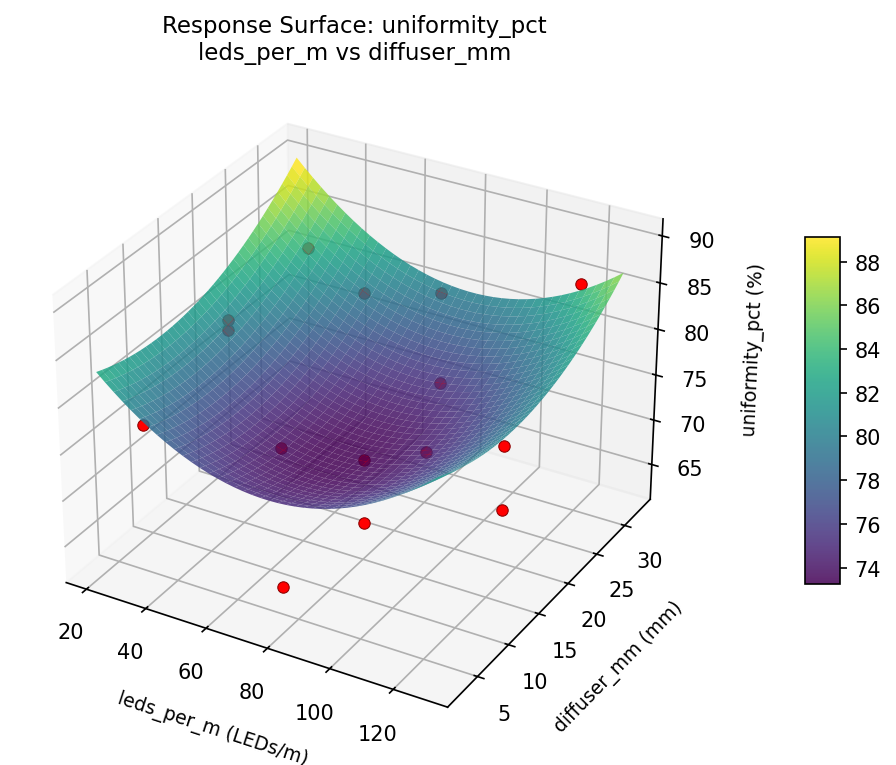
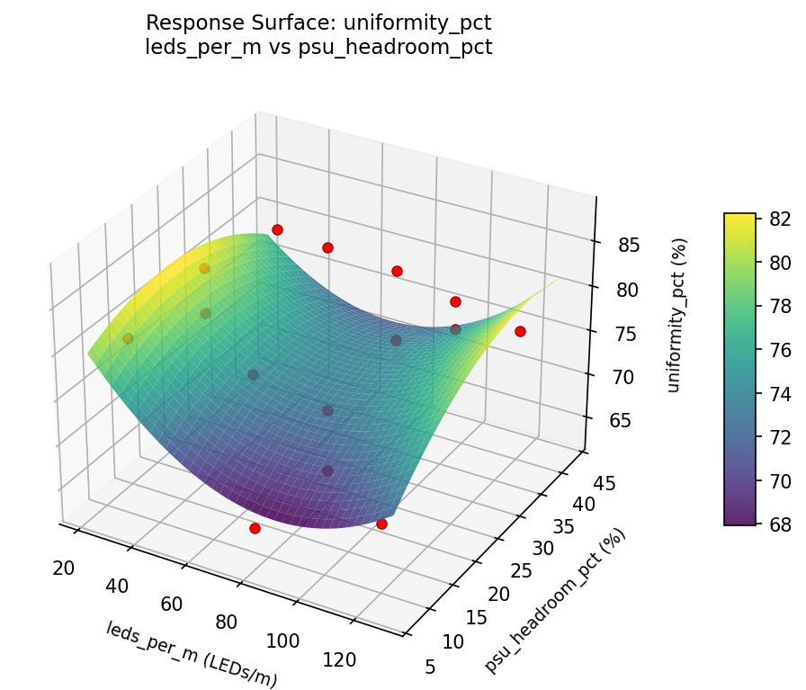
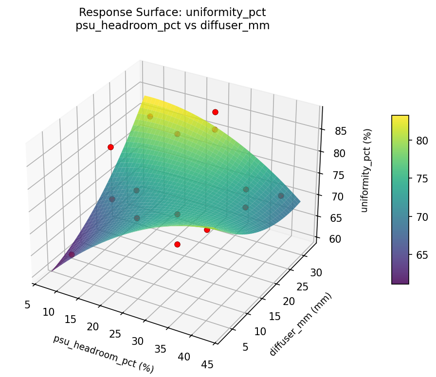
Response Surface Plots

3D surfaces fitted with quadratic RSM. Red dots are observed data points.

hotspot temp c leds per m vs diffuser mm

hotspot temp c leds per m vs psu headroom pct

hotspot temp c psu headroom pct vs diffuser mm

uniformity pct leds per m vs diffuser mm

uniformity pct leds per m vs psu headroom pct

uniformity pct psu headroom pct vs diffuser mm

Multi-Objective Optimization

When responses compete, Derringer–Suich desirability finds the best compromise. Each response is scaled to a 0–1 desirability, then combined via a weighted geometric mean.

Overall Desirability

D = 0.7271

Per-Response Desirability

Response	Weight	Desirability	Predicted	Dir
`uniformity_pct`	1.5	0.7727	83.00 0.7727 83.00 %	↑
`hotspot_temp_c`	1.0	0.6636	32.00 0.6636 32.00 C	↓

Recommended Settings

Factor	Value
`leds_per_m`	75 LEDs/m
`psu_headroom_pct`	25 %
`diffuser_mm`	17.5 mm

Source: from observed run #12

Trade-off Summary

Sacrifice = how much worse than single-objective best.

Response	Predicted	Best Observed	Sacrifice
`hotspot_temp_c`	32.00	24.00	+8.00

Top 3 Runs by Desirability

Run	D	Factor Settings
#2	0.6377	leds_per_m=75, psu_headroom_pct=25, diffuser_mm=17.5
#5	0.6377	leds_per_m=75, psu_headroom_pct=10, diffuser_mm=5

Model Quality

Response	R²	Type
`hotspot_temp_c`	0.3537	linear

Full Multi-Objective Output

doe optimize --multi
============================================================
MULTI-OBJECTIVE OPTIMIZATION
Method: Derringer-Suich Desirability Function
============================================================

Overall desirability: D = 0.7271

Response                  Weight Desirability    Predicted  Direction
---------------------------------------------------------------------
uniformity_pct               1.5       0.7727       83.00 %   ↑
hotspot_temp_c               1.0       0.6636       32.00 C   ↓

Recommended settings:
  leds_per_m = 75 LEDs/m
  psu_headroom_pct = 25 %
  diffuser_mm = 17.5 mm
  (from observed run #12)

Trade-off summary:
  uniformity_pct: 83.00 (best observed: 88.00, sacrifice: +5.00)
  hotspot_temp_c: 32.00 (best observed: 24.00, sacrifice: +8.00)

Model quality:
  uniformity_pct: R² = 0.8881 (quadratic)
  hotspot_temp_c: R² = 0.3537 (linear)

Top 3 observed runs by overall desirability:
  1. Run #12 (D=0.7271): leds_per_m=75, psu_headroom_pct=25, diffuser_mm=17.5
  2. Run #2 (D=0.6377): leds_per_m=75, psu_headroom_pct=25, diffuser_mm=17.5
  3. Run #5 (D=0.6377): leds_per_m=75, psu_headroom_pct=10, diffuser_mm=5

Full Analysis Output

doe analyze
=== Main Effects: uniformity_pct ===
Factor                   Effect    Std Error   % Contribution
--------------------------------------------------------------
leds_per_m              12.3571       1.9777            75.2%
psu_headroom_pct         2.5714       1.9777            15.7%
diffuser_mm              1.5000       1.9777             9.1%

=== ANOVA Table: uniformity_pct ===
Source                      DF           SS           MS          F    p-value
-----------------------------------------------------------------------------
leds_per_m                   2     392.4762     196.2381      7.452     0.0149
psu_headroom_pct             2      20.6190      10.3095      0.392     0.6883
diffuser_mm                  2       4.9762       2.4881      0.094     0.9108
Lack of Fit                  6     350.5952      58.4325      2.219     0.3429
Pure Error                   2      52.6667      26.3333
Error                        8     403.2619      26.3333
Total                       14     821.3333      58.6667

=== Summary Statistics: uniformity_pct ===

leds_per_m:
  Level               N       Mean        Std        Min        Max
  ------------------------------------------------------------
  120                 4    77.5000     9.0370    69.0000    88.0000
  30                  4    68.5000     6.4550    63.0000    77.0000
  75                  7    80.8571     3.1320    76.0000    86.0000

psu_headroom_pct:
  Level               N       Mean        Std        Min        Max
  ------------------------------------------------------------
  10                  4    78.0000    10.6145    63.0000    88.0000
  25                  7    75.4286     6.0238    69.0000    86.0000
  40                  4    77.5000     9.0370    64.0000    83.0000

diffuser_mm:
  Level               N       Mean        Std        Min        Max
  ------------------------------------------------------------
  17.5                7    76.8571     9.9738    63.0000    88.0000
  30                  4    77.2500     4.5000    71.0000    81.0000
  5                   4    75.7500     7.2744    69.0000    83.0000

=== Main Effects: hotspot_temp_c ===
Factor                   Effect    Std Error   % Contribution
--------------------------------------------------------------
psu_headroom_pct         5.0000       1.8809            38.0%
diffuser_mm              4.5000       1.8809            34.2%
leds_per_m               3.6429       1.8809            27.7%

=== ANOVA Table: hotspot_temp_c ===
Source                      DF           SS           MS          F    p-value
-----------------------------------------------------------------------------
leds_per_m                   2      34.0762      17.0381      0.412     0.6755
psu_headroom_pct             2      50.0048      25.0024      0.605     0.5693
diffuser_mm                  2      41.4333      20.7167      0.501     0.6236
Lack of Fit                  6     534.7524      89.1254      2.156     0.3503
Pure Error                   2      82.6667      41.3333
Error                        8     617.4190      41.3333
Total                       14     742.9333      53.0667

=== Summary Statistics: hotspot_temp_c ===

leds_per_m:
  Level               N       Mean        Std        Min        Max
  ------------------------------------------------------------
  120                 4    36.5000     8.7369    24.0000    43.0000
  30                  4    34.5000     8.5829    28.0000    47.0000
  75                  7    38.1429     6.5683    32.0000    49.0000

psu_headroom_pct:
  Level               N       Mean        Std        Min        Max
  ------------------------------------------------------------
  10                  4    39.2500     8.4212    30.0000    49.0000
  25                  7    36.7143     8.8075    24.0000    47.0000
  40                  4    34.2500     2.2174    32.0000    37.0000

diffuser_mm:
  Level               N       Mean        Std        Min        Max
  ------------------------------------------------------------
  17.5                7    37.0000     5.6569    30.0000    46.0000
  30                  4    38.7500    11.6154    24.0000    49.0000
  5                   4    34.2500     5.9090    28.0000    42.0000

Optimization Recommendations

doe optimize
=== Optimization: uniformity_pct ===
Direction: maximize

Best observed run: #3
  leds_per_m = 120
  psu_headroom_pct = 25
  diffuser_mm = 30
  Value: 88.0

RSM Model (linear, R² = 0.0944, Adj R² = -0.1526):
  Coefficients:
    intercept                      +76.6667
    leds_per_m                     +0.7500
    psu_headroom_pct               +2.7500
    diffuser_mm                    +1.2500

RSM Model (quadratic, R² = 0.4756, Adj R² = -0.4682):
  Coefficients:
    intercept                      +75.6667
    leds_per_m                     +0.7500
    psu_headroom_pct               +2.7500
    diffuser_mm                    +1.2500
    leds_per_m*psu_headroom_pct    -0.7500
    leds_per_m*diffuser_mm         +6.7500
    psu_headroom_pct*diffuser_mm   +3.7500
    leds_per_m^2                   +2.7917
    psu_headroom_pct^2             -2.7083
    diffuser_mm^2                  +1.7917

  Curvature analysis:
    leds_per_m                     coef=+2.7917  convex (has a minimum)
    psu_headroom_pct               coef=-2.7083  concave (has a maximum)
    diffuser_mm                    coef=+1.7917  convex (has a minimum)

  Notable interactions:
    leds_per_m*diffuser_mm         coef=+6.7500  (synergistic)
    psu_headroom_pct*diffuser_mm   coef=+3.7500  (synergistic)
    leds_per_m*psu_headroom_pct    coef=-0.7500  (antagonistic)

  Predicted optimum (from linear model, at observed points):
    leds_per_m = 75
    psu_headroom_pct = 40
    diffuser_mm = 30
    Predicted value: 80.6667

  Surface optimum (via L-BFGS-B, linear model):
    leds_per_m = 120
    psu_headroom_pct = 40
    diffuser_mm = 30
    Predicted value: 81.4167

  Model quality: Weak fit — consider adding center points or using a different design.

Factor importance:
  1. psu_headroom_pct  (effect: 5.8, contribution: 46.6%)
  2. leds_per_m  (effect: 3.6, contribution: 29.0%)
  3. diffuser_mm  (effect: 3.0, contribution: 24.4%)

=== Optimization: hotspot_temp_c ===
Direction: minimize

Best observed run: #14
  leds_per_m = 30
  psu_headroom_pct = 40
  diffuser_mm = 17.5
  Value: 24.0

RSM Model (linear, R² = 0.0448, Adj R² = -0.2158):
  Coefficients:
    intercept                      +36.7333
    leds_per_m                     +0.5000
    psu_headroom_pct               -1.6250
    diffuser_mm                    -1.1250

RSM Model (quadratic, R² = 0.5048, Adj R² = -0.3866):
  Coefficients:
    intercept                      +41.3333
    leds_per_m                     +0.5000
    psu_headroom_pct               -1.6250
    diffuser_mm                    -1.1250
    leds_per_m*psu_headroom_pct    +4.0000
    leds_per_m*diffuser_mm         +6.0000
    psu_headroom_pct*diffuser_mm   +0.7500
    leds_per_m^2                   -1.0417
    psu_headroom_pct^2             -5.7917
    diffuser_mm^2                  -1.7917

  Curvature analysis:
    psu_headroom_pct               coef=-5.7917  concave (has a maximum)
    diffuser_mm                    coef=-1.7917  concave (has a maximum)
    leds_per_m                     coef=-1.0417  concave (has a maximum)

  Notable interactions:
    leds_per_m*diffuser_mm         coef=+6.0000  (synergistic)
    leds_per_m*psu_headroom_pct    coef=+4.0000  (synergistic)
    psu_headroom_pct*diffuser_mm   coef=+0.7500  (synergistic)

  Predicted optimum (from linear model, at observed points):
    leds_per_m = 75
    psu_headroom_pct = 10
    diffuser_mm = 5
    Predicted value: 39.4833

  Surface optimum (via L-BFGS-B, linear model):
    leds_per_m = 30
    psu_headroom_pct = 40
    diffuser_mm = 30
    Predicted value: 33.4833

  Model quality: Weak fit — consider adding center points or using a different design.

Factor importance:
  1. psu_headroom_pct  (effect: 7.2, contribution: 67.8%)
  2. diffuser_mm  (effect: 2.4, contribution: 22.8%)
  3. leds_per_m  (effect: 1.0, contribution: 9.4%)