Summary
This experiment investigates battery charger settings. Full factorial of charge current, voltage cutoff, trickle threshold, and temperature limit to maximize capacity and cycle life.
The design varies 4 factors: charge c (C), ranging from 0.5 to 2.0, cutoff v (V), ranging from 4.15 to 4.25, trickle pct (%), ranging from 3 to 10, and temp limit c (C), ranging from 35 to 50. The goal is to optimize 2 responses: capacity pct (%) (maximize) and cycle life (cycles) (maximize). Fixed conditions held constant across all runs include chemistry = LiPo, cells = 3S.
A full factorial design was used to explore all 16 possible combinations of the 4 factors at two levels. This guarantees that every main effect and interaction can be estimated independently, at the cost of a larger experiment (16 runs).
Quadratic response surface models were fitted to capture potential curvature and factor interactions. The RSM contour plots below visualize how pairs of factors jointly affect each response.
Key Findings
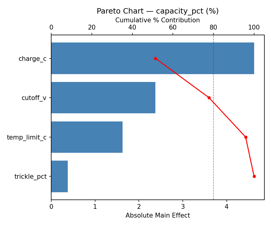
For capacity pct, the most influential factors were cutoff v (38.8%), trickle pct (30.2%), temp limit c (21.6%). The best observed value was 99.0 (at charge c = 0.5, cutoff v = 4.25, trickle pct = 3).
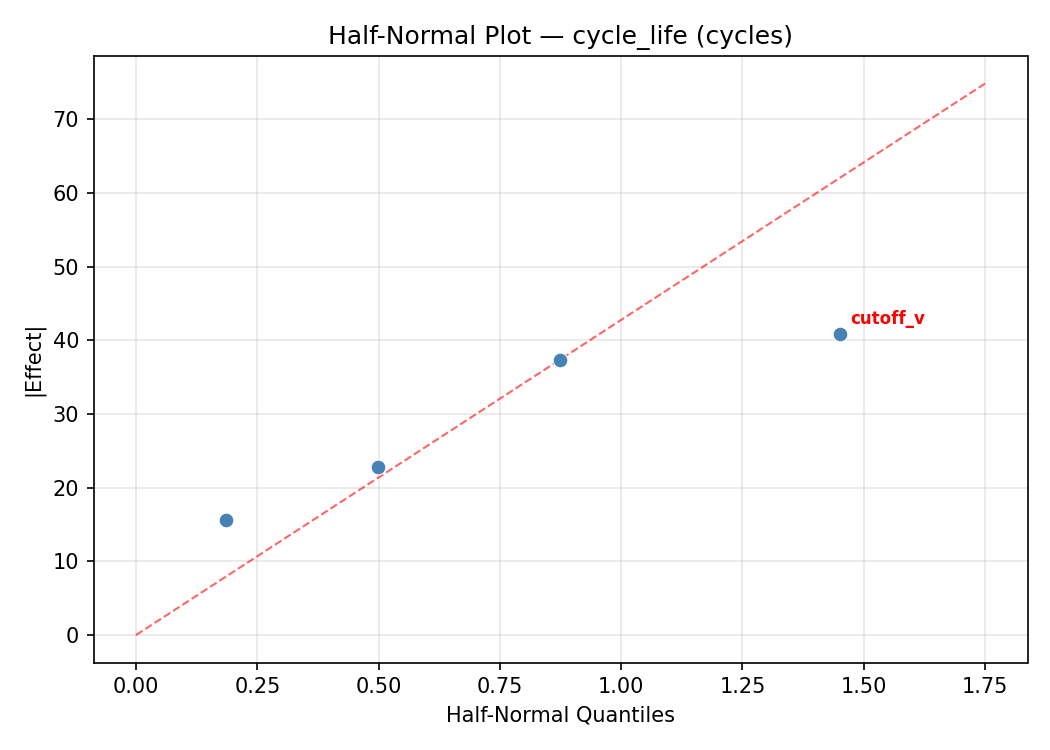
For cycle life, the most influential factors were trickle pct (33.5%), cutoff v (28.5%), temp limit c (20.4%). The best observed value was 745.0 (at charge c = 2.0, cutoff v = 4.25, trickle pct = 3).
Recommended Next Steps
- Consider whether any fixed factors should be varied in a future study.
Experimental Setup
Factors
| Factor | Low | High | Unit |
|---|
charge_c | 0.5 | 2.0 | C |
cutoff_v | 4.15 | 4.25 | V |
trickle_pct | 3 | 10 | % |
temp_limit_c | 35 | 50 | C |
Fixed: chemistry = LiPo, cells = 3S
Responses
| Response | Direction | Unit |
|---|
capacity_pct | ↑ maximize | % |
cycle_life | ↑ maximize | cycles |
Configuration
{
"metadata": {
"name": "Battery Charger Settings",
"description": "Full factorial of charge current, voltage cutoff, trickle threshold, and temperature limit to maximize capacity and cycle life"
},
"factors": [
{
"name": "charge_c",
"levels": [
"0.5",
"2.0"
],
"type": "continuous",
"unit": "C"
},
{
"name": "cutoff_v",
"levels": [
"4.15",
"4.25"
],
"type": "continuous",
"unit": "V"
},
{
"name": "trickle_pct",
"levels": [
"3",
"10"
],
"type": "continuous",
"unit": "%"
},
{
"name": "temp_limit_c",
"levels": [
"35",
"50"
],
"type": "continuous",
"unit": "C"
}
],
"fixed_factors": {
"chemistry": "LiPo",
"cells": "3S"
},
"responses": [
{
"name": "capacity_pct",
"optimize": "maximize",
"unit": "%"
},
{
"name": "cycle_life",
"optimize": "maximize",
"unit": "cycles"
}
],
"settings": {
"operation": "full_factorial",
"test_script": "use_cases/274_battery_charger/sim.sh"
}
}
Experimental Matrix
The Full Factorial Design produces 16 runs. Each row is one experiment with specific factor settings.
| Run | charge_c | cutoff_v | trickle_pct | temp_limit_c |
|---|
| 1 | 0.5 | 4.25 | 10 | 50 |
| 2 | 2.0 | 4.15 | 3 | 50 |
| 3 | 0.5 | 4.25 | 3 | 50 |
| 4 | 0.5 | 4.25 | 10 | 35 |
| 5 | 2.0 | 4.25 | 10 | 35 |
| 6 | 2.0 | 4.15 | 10 | 35 |
| 7 | 2.0 | 4.25 | 3 | 35 |
| 8 | 2.0 | 4.15 | 3 | 35 |
| 9 | 0.5 | 4.15 | 3 | 50 |
| 10 | 0.5 | 4.15 | 10 | 35 |
| 11 | 2.0 | 4.25 | 3 | 50 |
| 12 | 2.0 | 4.25 | 10 | 50 |
| 13 | 0.5 | 4.25 | 3 | 35 |
| 14 | 2.0 | 4.15 | 10 | 50 |
| 15 | 0.5 | 4.15 | 3 | 35 |
| 16 | 0.5 | 4.15 | 10 | 50 |
Step-by-Step Workflow
1
Preview the design
$ doe info --config use_cases/274_battery_charger/config.json
2
Generate the runner script
$ doe generate --config use_cases/274_battery_charger/config.json \
--output use_cases/274_battery_charger/results/run.sh --seed 42
3
Execute the experiments
$ bash use_cases/274_battery_charger/results/run.sh
4
Analyze results
$ doe analyze --config use_cases/274_battery_charger/config.json
5
Get optimization recommendations
$ doe optimize --config use_cases/274_battery_charger/config.json
6
Multi-objective optimization
With 2 competing responses, use --multi to find the best compromise via Derringer–Suich desirability.
$ doe optimize --config use_cases/274_battery_charger/config.json --multi
7
Generate the HTML report
$ doe report --config use_cases/274_battery_charger/config.json \
--output use_cases/274_battery_charger/results/report.html
Features Exercised
| Feature | Value |
|---|
| Design type | full_factorial |
| Factor types | continuous (all 4) |
| Arg style | double-dash |
| Responses | 2 (capacity_pct ↑, cycle_life ↑) |
| Total runs | 16 |
Analysis Results
Generated from actual experiment runs using the DOE Helper Tool.
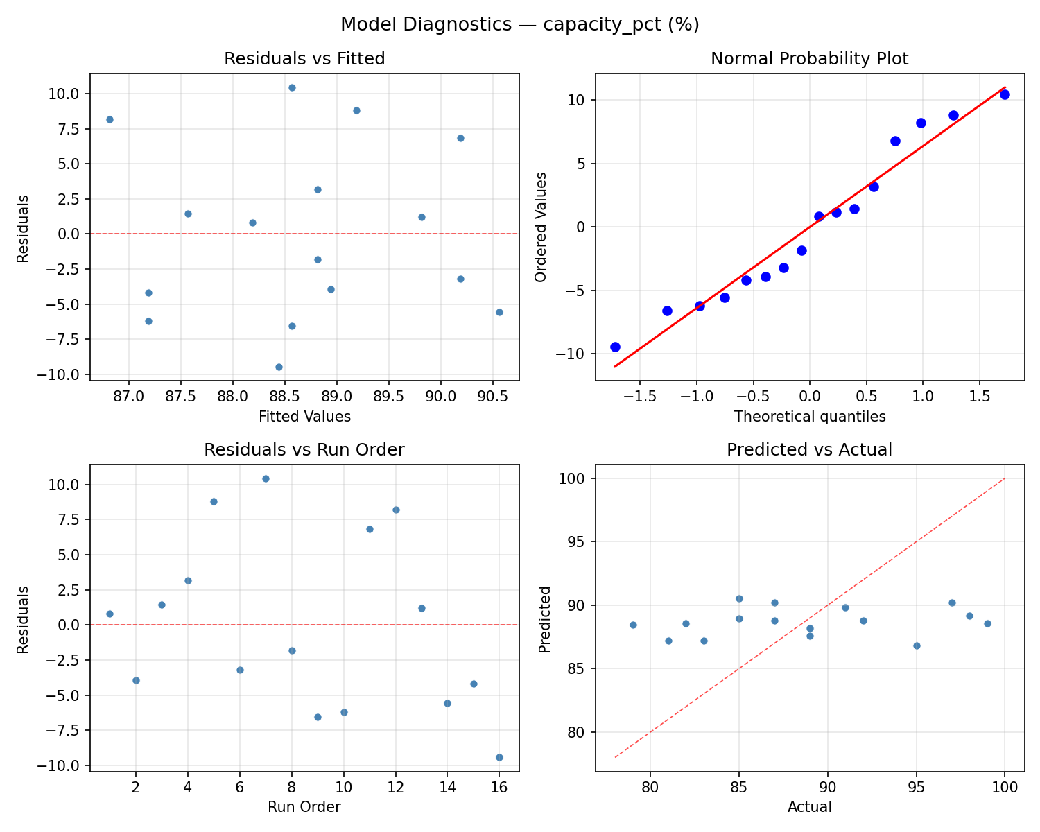
Response: capacity_pct
Top factors: cutoff_v (38.8%), trickle_pct (30.2%), temp_limit_c (21.6%).
ANOVA
| Source | DF | SS | MS | F | p-value |
|---|
| Source | DF | SS | MS | F | p-value |
| charge_c | 1 | 7.5625 | 7.5625 | 0.185 | 0.6853 |
| cutoff_v | 1 | 126.5625 | 126.5625 | 3.090 | 0.1391 |
| trickle_pct | 1 | 76.5625 | 76.5625 | 1.869 | 0.2298 |
| temp_limit_c | 1 | 39.0625 | 39.0625 | 0.954 | 0.3736 |
| charge_c*cutoff_v | 1 | 33.0625 | 33.0625 | 0.807 | 0.4101 |
| charge_c*trickle_pct | 1 | 1.5625 | 1.5625 | 0.038 | 0.8528 |
| charge_c*temp_limit_c | 1 | 27.5625 | 27.5625 | 0.673 | 0.4494 |
| cutoff_v*trickle_pct | 1 | 39.0625 | 39.0625 | 0.954 | 0.3736 |
| cutoff_v*temp_limit_c | 1 | 3.0625 | 3.0625 | 0.075 | 0.7955 |
| trickle_pct*temp_limit_c | 1 | 22.5625 | 22.5625 | 0.551 | 0.4914 |
| Error | 5 | 204.8125 | 40.9625 | | |
| Total | 15 | 581.4375 | 38.7625 | | |
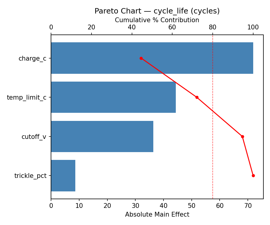
Pareto Chart
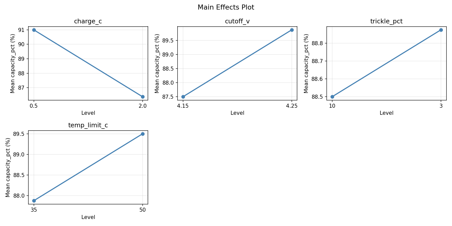
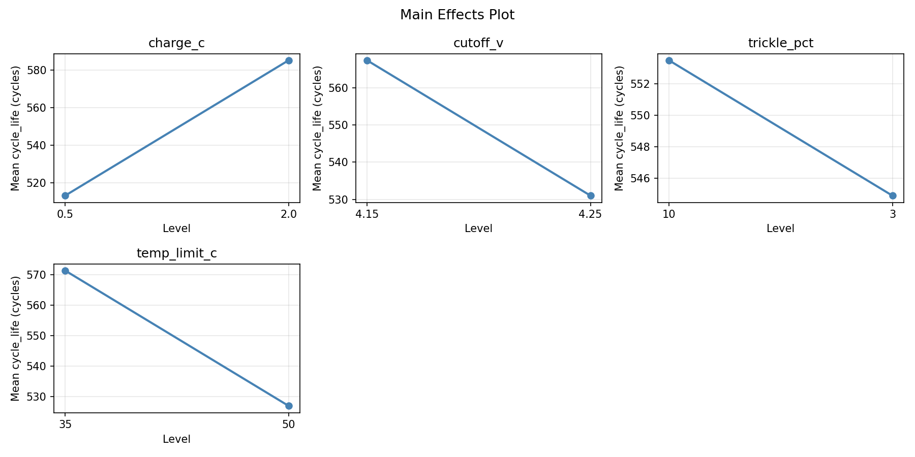
Main Effects Plot
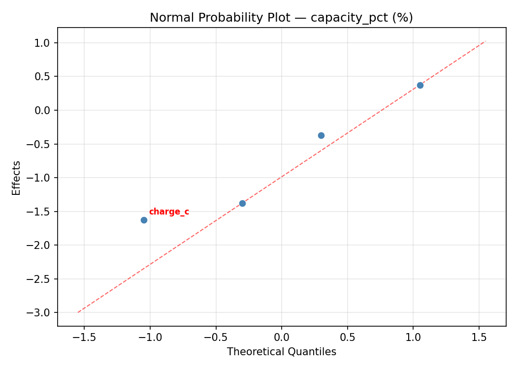
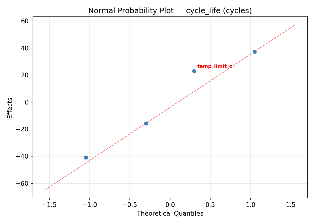
Normal Probability Plot of Effects
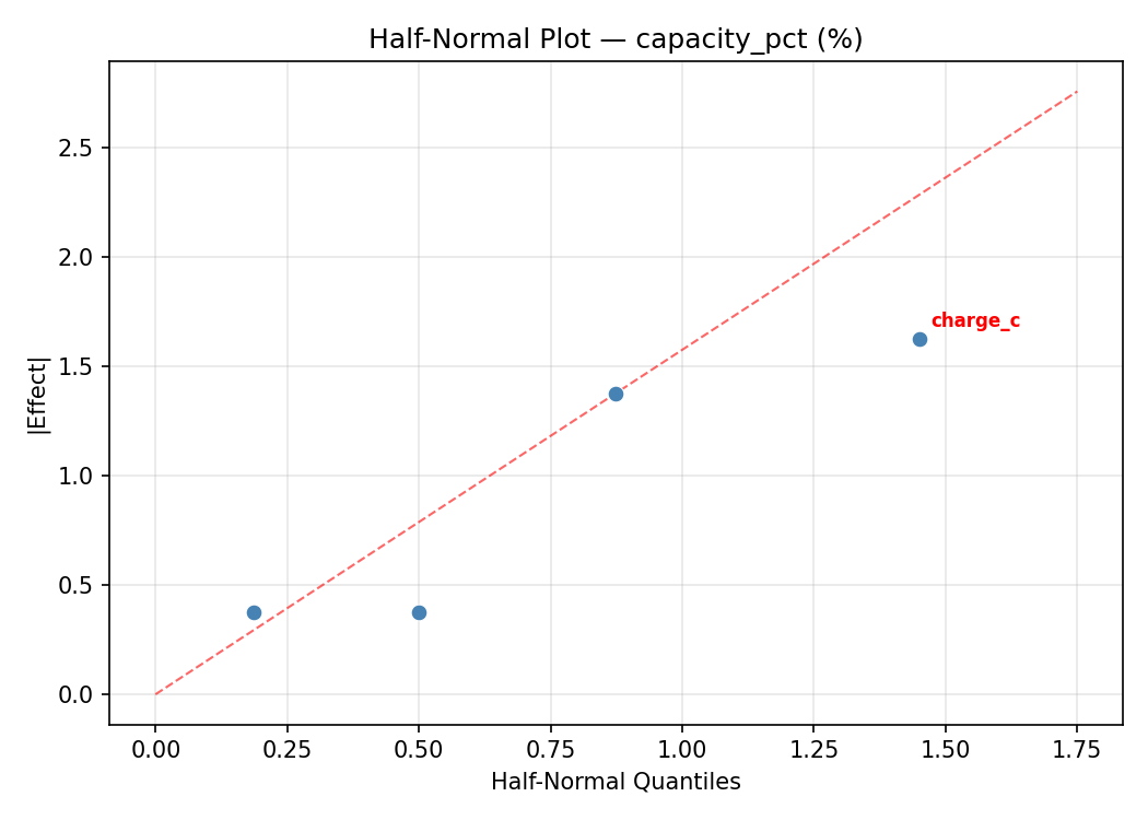
Half-Normal Plot of Effects
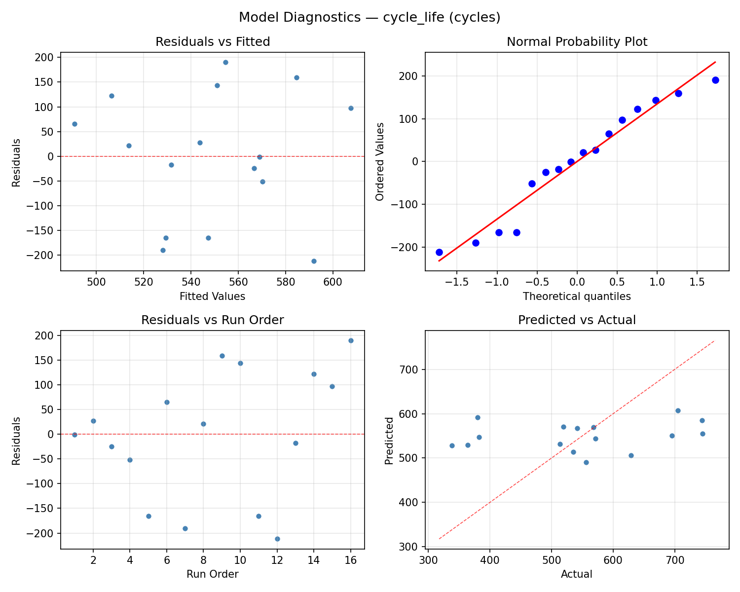
Model Diagnostics
Response: cycle_life
Top factors: trickle_pct (33.5%), cutoff_v (28.5%), temp_limit_c (20.4%).
ANOVA
| Source | DF | SS | MS | F | p-value |
|---|
| Source | DF | SS | MS | F | p-value |
| charge_c | 1 | 15562.5625 | 15562.5625 | 1.073 | 0.3478 |
| cutoff_v | 1 | 41107.5625 | 41107.5625 | 2.834 | 0.1531 |
| trickle_pct | 1 | 56763.0625 | 56763.0625 | 3.913 | 0.1048 |
| temp_limit_c | 1 | 20952.5625 | 20952.5625 | 1.444 | 0.2833 |
| charge_c*cutoff_v | 1 | 18428.0625 | 18428.0625 | 1.270 | 0.3109 |
| charge_c*trickle_pct | 1 | 264.0625 | 264.0625 | 0.018 | 0.8979 |
| charge_c*temp_limit_c | 1 | 9653.0625 | 9653.0625 | 0.665 | 0.4518 |
| cutoff_v*trickle_pct | 1 | 13398.0625 | 13398.0625 | 0.924 | 0.3807 |
| cutoff_v*temp_limit_c | 1 | 798.0625 | 798.0625 | 0.055 | 0.8239 |
| trickle_pct*temp_limit_c | 1 | 17490.0625 | 17490.0625 | 1.206 | 0.3222 |
| Error | 5 | 72535.3125 | 14507.0625 | | |
| Total | 15 | 266952.4375 | 17796.8292 | | |
Pareto Chart
Main Effects Plot
Normal Probability Plot of Effects
Half-Normal Plot of Effects
Model Diagnostics
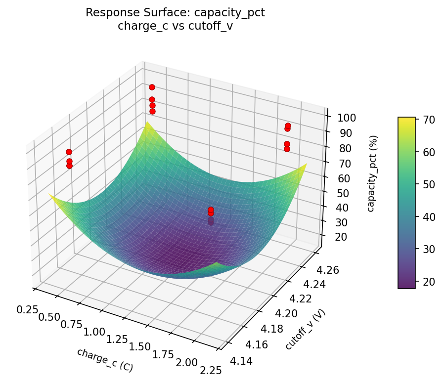
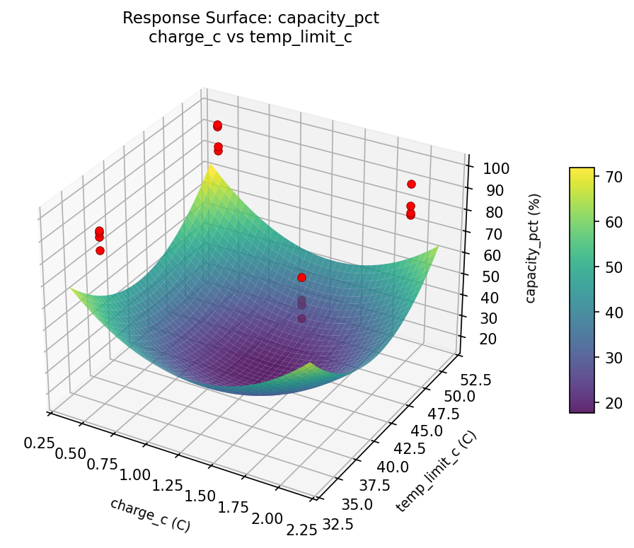
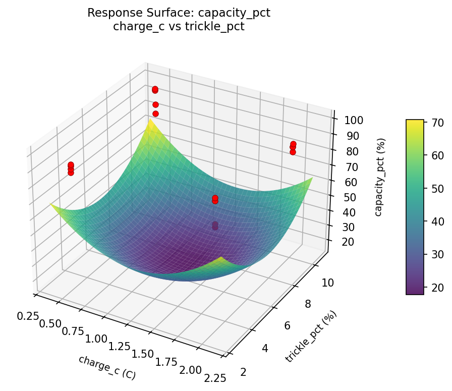
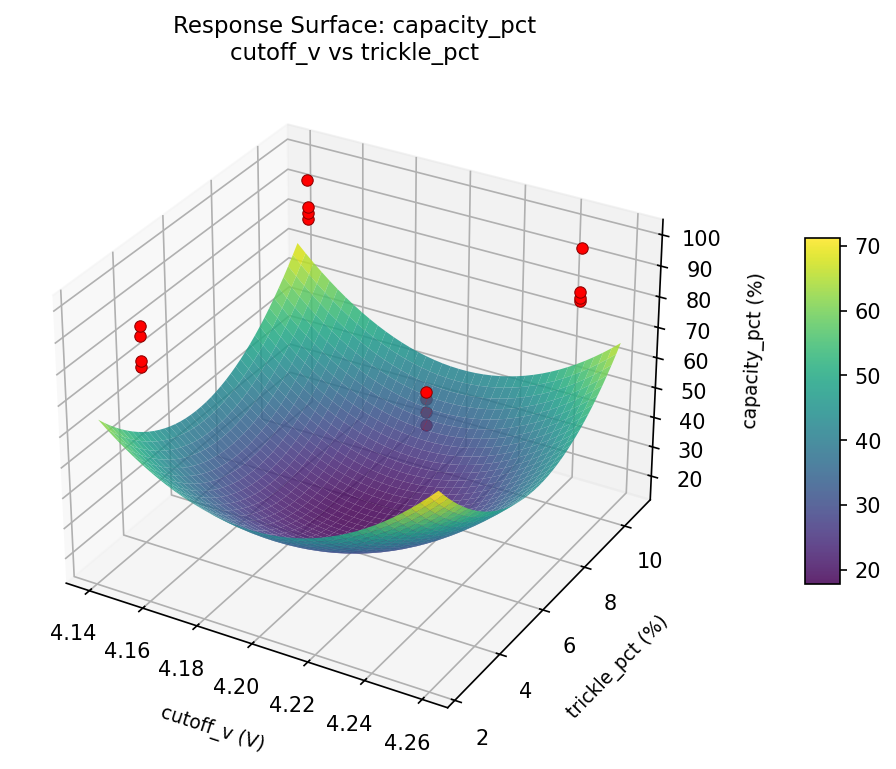
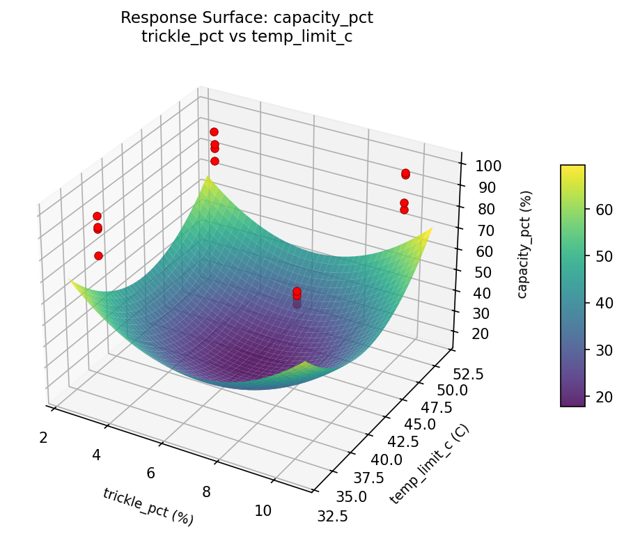
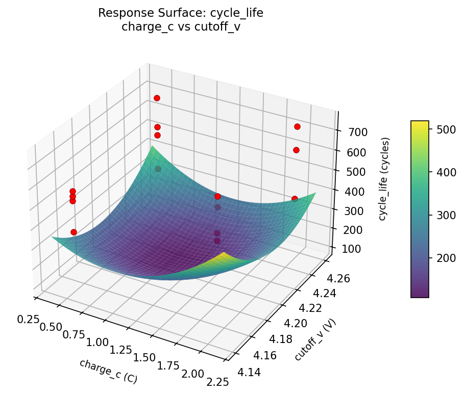
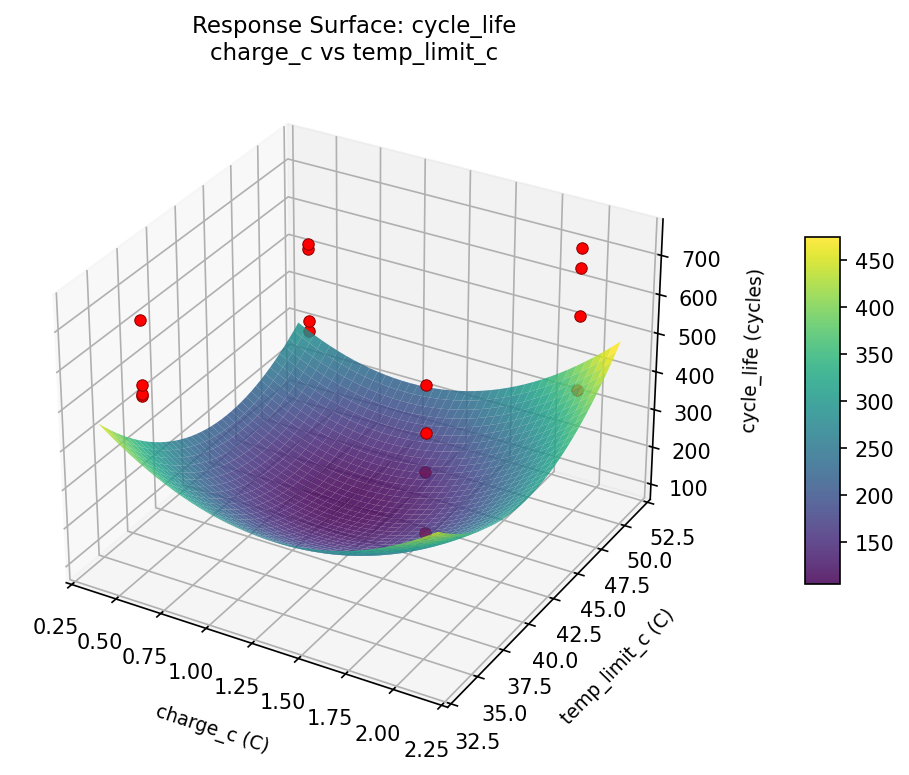
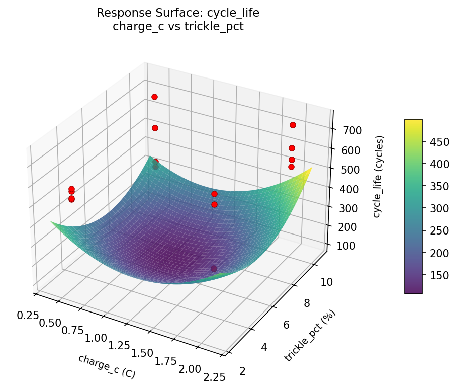
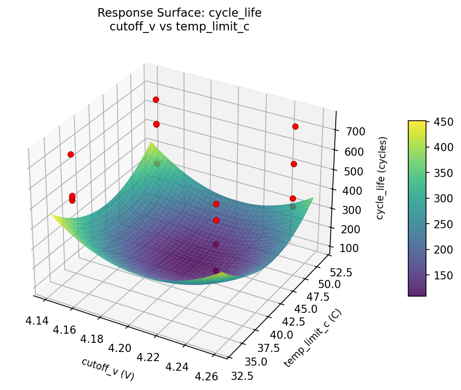
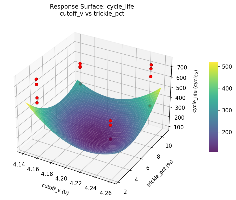
Response Surface Plots
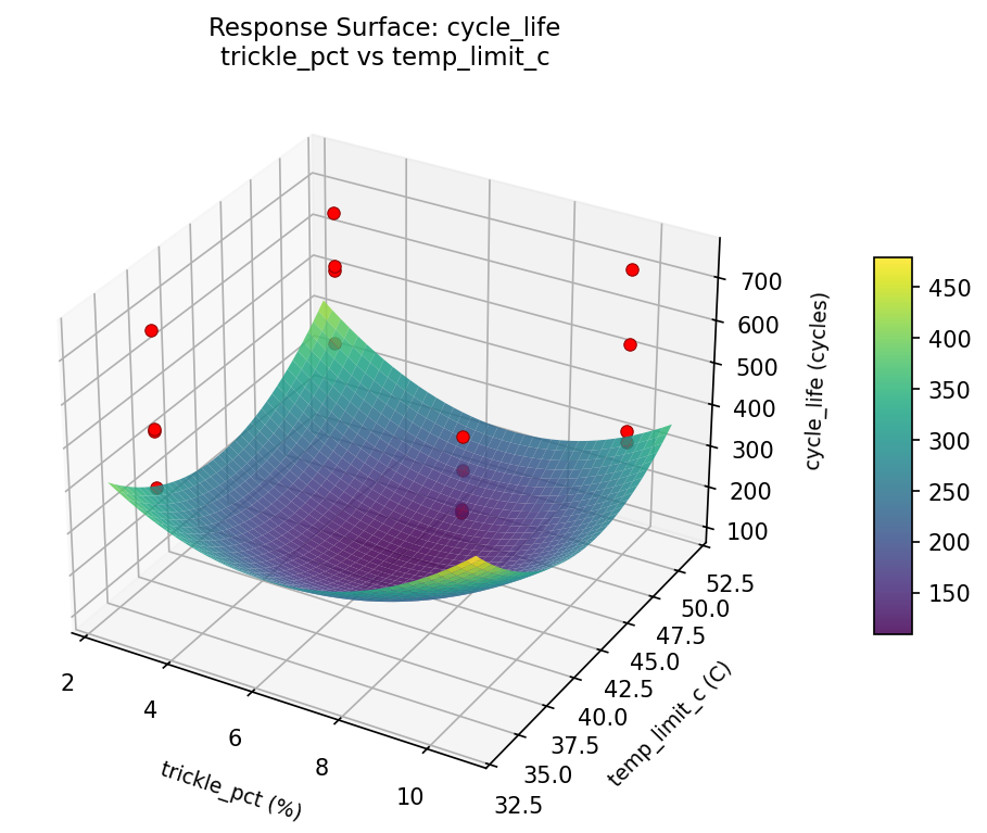
3D surfaces fitted with quadratic RSM. Red dots are observed data points.
capacity pct charge c vs cutoff v
capacity pct charge c vs temp limit c
capacity pct charge c vs trickle pct
capacity pct cutoff v vs temp limit c

capacity pct cutoff v vs trickle pct
capacity pct trickle pct vs temp limit c
cycle life charge c vs cutoff v
cycle life charge c vs temp limit c
cycle life charge c vs trickle pct
cycle life cutoff v vs temp limit c
cycle life cutoff v vs trickle pct
cycle life trickle pct vs temp limit c
Multi-Objective Optimization
When responses compete, Derringer–Suich desirability finds the best compromise.
Each response is scaled to a 0–1 desirability, then combined via a weighted geometric mean.
Overall Desirability
D = 0.5350
Per-Response Desirability
| Response | Weight | Desirability | Predicted | Dir |
|---|
capacity_pct |
1.5 |
|
92.00 0.6364 92.00 % |
↑ |
cycle_life |
1.5 |
|
519.00 0.4497 519.00 cycles |
↑ |
Recommended Settings
| Factor | Value |
|---|
charge_c | 2.0 C |
cutoff_v | 4.15 V |
trickle_pct | 3 % |
temp_limit_c | 35 C |
Source: from observed run #4
Trade-off Summary
Sacrifice = how much worse than single-objective best.
| Response | Predicted | Best Observed | Sacrifice |
|---|
cycle_life | 519.00 | 745.00 | +226.00 |
Top 3 Runs by Desirability
| Run | D | Factor Settings |
|---|
| #1 | 0.5288 | charge_c=2.0, cutoff_v=4.25, trickle_pct=3, temp_limit_c=50 |
| #13 | 0.5091 | charge_c=0.5, cutoff_v=4.25, trickle_pct=3, temp_limit_c=50 |
Model Quality
| Response | R² | Type |
|---|
cycle_life | 0.5582 | linear |
Full Multi-Objective Output
============================================================
MULTI-OBJECTIVE OPTIMIZATION
Method: Derringer-Suich Desirability Function
============================================================
Overall desirability: D = 0.5350
Response Weight Desirability Predicted Direction
---------------------------------------------------------------------
capacity_pct 1.5 0.6364 92.00 % ↑
cycle_life 1.5 0.4497 519.00 cycles ↑
Recommended settings:
charge_c = 2.0 C
cutoff_v = 4.15 V
trickle_pct = 3 %
temp_limit_c = 35 C
(from observed run #4)
Trade-off summary:
capacity_pct: 92.00 (best observed: 99.00, sacrifice: +7.00)
cycle_life: 519.00 (best observed: 745.00, sacrifice: +226.00)
Model quality:
capacity_pct: R² = 0.4244 (linear)
cycle_life: R² = 0.5582 (linear)
Top 3 observed runs by overall desirability:
1. Run #4 (D=0.5350): charge_c=2.0, cutoff_v=4.15, trickle_pct=3, temp_limit_c=35
2. Run #1 (D=0.5288): charge_c=2.0, cutoff_v=4.25, trickle_pct=3, temp_limit_c=50
3. Run #13 (D=0.5091): charge_c=0.5, cutoff_v=4.25, trickle_pct=3, temp_limit_c=50
Full Analysis Output
=== Main Effects: capacity_pct ===
Factor Effect Std Error % Contribution
--------------------------------------------------------------
cutoff_v 5.6250 1.5565 38.8%
trickle_pct -4.3750 1.5565 30.2%
temp_limit_c -3.1250 1.5565 21.6%
charge_c 1.3750 1.5565 9.5%
=== ANOVA Table: capacity_pct ===
Source DF SS MS F p-value
-----------------------------------------------------------------------------
charge_c 1 7.5625 7.5625 0.185 0.6853
cutoff_v 1 126.5625 126.5625 3.090 0.1391
trickle_pct 1 76.5625 76.5625 1.869 0.2298
temp_limit_c 1 39.0625 39.0625 0.954 0.3736
charge_c*cutoff_v 1 33.0625 33.0625 0.807 0.4101
charge_c*trickle_pct 1 1.5625 1.5625 0.038 0.8528
charge_c*temp_limit_c 1 27.5625 27.5625 0.673 0.4494
cutoff_v*trickle_pct 1 39.0625 39.0625 0.954 0.3736
cutoff_v*temp_limit_c 1 3.0625 3.0625 0.075 0.7955
trickle_pct*temp_limit_c 1 22.5625 22.5625 0.551 0.4914
Error 5 204.8125 40.9625
Total 15 581.4375 38.7625
=== Interaction Effects: capacity_pct ===
Factor A Factor B Interaction % Contribution
------------------------------------------------------------------------
cutoff_v trickle_pct -3.1250 25.0%
charge_c cutoff_v -2.8750 23.0%
charge_c temp_limit_c -2.6250 21.0%
trickle_pct temp_limit_c -2.3750 19.0%
cutoff_v temp_limit_c -0.8750 7.0%
charge_c trickle_pct 0.6250 5.0%
=== Summary Statistics: capacity_pct ===
charge_c:
Level N Mean Std Min Max
------------------------------------------------------------
0.5 8 88.0000 5.7817 79.0000 97.0000
2.0 8 89.3750 6.9680 81.0000 99.0000
cutoff_v:
Level N Mean Std Min Max
------------------------------------------------------------
4.15 8 85.8750 6.2206 79.0000 99.0000
4.25 8 91.5000 5.1270 83.0000 98.0000
trickle_pct:
Level N Mean Std Min Max
------------------------------------------------------------
10 8 90.8750 5.2491 85.0000 98.0000
3 8 86.5000 6.6762 79.0000 99.0000
temp_limit_c:
Level N Mean Std Min Max
------------------------------------------------------------
35 8 90.2500 7.3436 79.0000 99.0000
50 8 87.1250 4.8532 81.0000 95.0000
=== Main Effects: cycle_life ===
Factor Effect Std Error % Contribution
--------------------------------------------------------------
trickle_pct 119.1250 33.3512 33.5%
cutoff_v -101.3750 33.3512 28.5%
temp_limit_c 72.3750 33.3512 20.4%
charge_c -62.3750 33.3512 17.6%
=== ANOVA Table: cycle_life ===
Source DF SS MS F p-value
-----------------------------------------------------------------------------
charge_c 1 15562.5625 15562.5625 1.073 0.3478
cutoff_v 1 41107.5625 41107.5625 2.834 0.1531
trickle_pct 1 56763.0625 56763.0625 3.913 0.1048
temp_limit_c 1 20952.5625 20952.5625 1.444 0.2833
charge_c*cutoff_v 1 18428.0625 18428.0625 1.270 0.3109
charge_c*trickle_pct 1 264.0625 264.0625 0.018 0.8979
charge_c*temp_limit_c 1 9653.0625 9653.0625 0.665 0.4518
cutoff_v*trickle_pct 1 13398.0625 13398.0625 0.924 0.3807
cutoff_v*temp_limit_c 1 798.0625 798.0625 0.055 0.8239
trickle_pct*temp_limit_c 1 17490.0625 17490.0625 1.206 0.3222
Error 5 72535.3125 14507.0625
Total 15 266952.4375 17796.8292
=== Interaction Effects: cycle_life ===
Factor A Factor B Interaction % Contribution
------------------------------------------------------------------------
charge_c cutoff_v 67.8750 25.8%
trickle_pct temp_limit_c 66.1250 25.1%
cutoff_v trickle_pct 57.8750 22.0%
charge_c temp_limit_c 49.1250 18.7%
cutoff_v temp_limit_c 14.1250 5.4%
charge_c trickle_pct -8.1250 3.1%
=== Summary Statistics: cycle_life ===
charge_c:
Level N Mean Std Min Max
------------------------------------------------------------
0.5 8 580.3750 122.7017 382.0000 745.0000
2.0 8 518.0000 144.4200 338.0000 705.0000
cutoff_v:
Level N Mean Std Min Max
------------------------------------------------------------
4.15 8 599.8750 135.5944 338.0000 745.0000
4.25 8 498.5000 117.8037 364.0000 705.0000
trickle_pct:
Level N Mean Std Min Max
------------------------------------------------------------
10 8 489.6250 100.5882 364.0000 629.0000
3 8 608.7500 141.0995 338.0000 745.0000
temp_limit_c:
Level N Mean Std Min Max
------------------------------------------------------------
35 8 513.0000 142.6865 338.0000 745.0000
50 8 585.3750 121.5870 380.0000 744.0000
Optimization Recommendations
=== Optimization: capacity_pct ===
Direction: maximize
Best observed run: #7
charge_c = 0.5
cutoff_v = 4.25
trickle_pct = 3
temp_limit_c = 50
Value: 99.0
RSM Model (linear, R² = 0.1268, Adj R² = -0.1907):
Coefficients:
intercept +88.6875
charge_c -0.3125
cutoff_v +0.0625
trickle_pct -1.4375
temp_limit_c -1.5625
RSM Model (quadratic, R² = 0.9780, Adj R² = 0.6695):
Coefficients:
intercept +17.7375
charge_c -0.3125
cutoff_v +0.0625
trickle_pct -1.4375
temp_limit_c -1.5625
charge_c*cutoff_v -3.4375
charge_c*trickle_pct +3.3125
charge_c*temp_limit_c -2.8125
cutoff_v*trickle_pct -0.3125
cutoff_v*temp_limit_c +0.3125
trickle_pct*temp_limit_c -0.1875
charge_c^2 +17.7375
cutoff_v^2 +17.7375
trickle_pct^2 +17.7375
temp_limit_c^2 +17.7375
Curvature analysis:
cutoff_v coef=+17.7375 convex (has a minimum)
trickle_pct coef=+17.7375 convex (has a minimum)
temp_limit_c coef=+17.7375 convex (has a minimum)
charge_c coef=+17.7375 convex (has a minimum)
Notable interactions:
charge_c*cutoff_v coef=-3.4375 (antagonistic)
charge_c*trickle_pct coef=+3.3125 (synergistic)
charge_c*temp_limit_c coef=-2.8125 (antagonistic)
cutoff_v*temp_limit_c coef=+0.3125 (synergistic)
cutoff_v*trickle_pct coef=-0.3125 (antagonistic)
Predicted optimum (from quadratic model, at observed points):
charge_c = 0.5
cutoff_v = 4.25
trickle_pct = 3
temp_limit_c = 50
Predicted value: 99.3125
Surface optimum (via L-BFGS-B, quadratic model):
charge_c = 0.5
cutoff_v = 4.25
trickle_pct = 3
temp_limit_c = 50
Predicted value: 99.3125
Model quality: Excellent fit — surface predictions are reliable.
Factor importance:
1. temp_limit_c (effect: -3.1, contribution: 46.3%)
2. trickle_pct (effect: 2.9, contribution: 42.6%)
3. charge_c (effect: -0.6, contribution: 9.3%)
4. cutoff_v (effect: 0.1, contribution: 1.9%)
=== Optimization: cycle_life ===
Direction: maximize
Best observed run: #16
charge_c = 2.0
cutoff_v = 4.25
trickle_pct = 3
temp_limit_c = 50
Value: 745.0
RSM Model (linear, R² = 0.2068, Adj R² = -0.0817):
Coefficients:
intercept +549.1875
charge_c -4.6875
cutoff_v +2.8125
trickle_pct +45.9375
temp_limit_c +36.1875
RSM Model (quadratic, R² = 0.9955, Adj R² = 0.9320):
Coefficients:
intercept +109.8375
charge_c -4.6875
cutoff_v +2.8125
trickle_pct +45.9375
temp_limit_c +36.1875
charge_c*cutoff_v +77.4375
charge_c*trickle_pct -59.1875
charge_c*temp_limit_c +60.0625
cutoff_v*trickle_pct +6.0625
cutoff_v*temp_limit_c +0.8125
trickle_pct*temp_limit_c -3.8125
charge_c^2 +109.8375
cutoff_v^2 +109.8375
trickle_pct^2 +109.8375
temp_limit_c^2 +109.8375
Curvature analysis:
charge_c coef=+109.8375 convex (has a minimum)
cutoff_v coef=+109.8375 convex (has a minimum)
temp_limit_c coef=+109.8375 convex (has a minimum)
trickle_pct coef=+109.8375 convex (has a minimum)
Notable interactions:
charge_c*cutoff_v coef=+77.4375 (synergistic)
charge_c*temp_limit_c coef=+60.0625 (synergistic)
charge_c*trickle_pct coef=-59.1875 (antagonistic)
cutoff_v*trickle_pct coef=+6.0625 (synergistic)
trickle_pct*temp_limit_c coef=-3.8125 (antagonistic)
cutoff_v*temp_limit_c coef=+0.8125 (synergistic)
Predicted optimum (from quadratic model, at observed points):
charge_c = 0.5
cutoff_v = 4.15
trickle_pct = 10
temp_limit_c = 35
Predicted value: 756.0625
Surface optimum (via L-BFGS-B, quadratic model):
charge_c = 0.5
cutoff_v = 4.15
trickle_pct = 10
temp_limit_c = 35
Predicted value: 756.0625
Model quality: Excellent fit — surface predictions are reliable.
Factor importance:
1. trickle_pct (effect: -91.9, contribution: 51.3%)
2. temp_limit_c (effect: 72.4, contribution: 40.4%)
3. charge_c (effect: -9.4, contribution: 5.2%)
4. cutoff_v (effect: 5.6, contribution: 3.1%)