Summary
This experiment investigates time-series downsampling. Central Composite design for downsampling interval, retention policy, and aggregation for query speed.
The design varies 3 factors: downsample interval m (min), ranging from 1 to 60, retention days (days), ranging from 7 to 365, and agg functions (count), ranging from 2 to 8. The goal is to optimize 2 responses: query p95 ms (ms) (minimize) and storage gb (GB) (minimize). Fixed conditions held constant across all runs include db engine = timescaledb, ingestion rate = 100000.
A Central Composite Design (CCD) was selected to fit a full quadratic response surface model, including curvature and interaction effects. With 3 factors this produces 22 runs including center points and axial (star) points that extend beyond the factorial range.
Quadratic response surface models were fitted to capture potential curvature and factor interactions. The RSM contour plots below visualize how pairs of factors jointly affect each response.
Key Findings
For query p95 ms, the most influential factors were retention days (44.9%), downsample interval m (35.4%), agg functions (19.7%). The best observed value was 6.0 (at downsample interval m = 1, retention days = 365, agg functions = 2).
For storage gb, the most influential factors were downsample interval m (43.6%), retention days (34.8%), agg functions (21.6%). The best observed value was 0.0 (at downsample interval m = 30.5, retention days = 512.808, agg functions = 5).
Recommended Next Steps
- Run confirmation experiments at the predicted optimal settings to validate the model.
- Consider whether any fixed factors should be varied in a future study.
Experimental Setup
Factors
| Factor | Low | High | Unit |
|---|
downsample_interval_m | 1 | 60 | min |
retention_days | 7 | 365 | days |
agg_functions | 2 | 8 | count |
Fixed: db_engine = timescaledb, ingestion_rate = 100000
Responses
| Response | Direction | Unit |
|---|
query_p95_ms | ↓ minimize | ms |
storage_gb | ↓ minimize | GB |
Configuration
{
"metadata": {
"name": "Time-Series Downsampling",
"description": "Central Composite design for downsampling interval, retention policy, and aggregation for query speed"
},
"factors": [
{
"name": "downsample_interval_m",
"levels": [
"1",
"60"
],
"type": "continuous",
"unit": "min"
},
{
"name": "retention_days",
"levels": [
"7",
"365"
],
"type": "continuous",
"unit": "days"
},
{
"name": "agg_functions",
"levels": [
"2",
"8"
],
"type": "continuous",
"unit": "count"
}
],
"fixed_factors": {
"db_engine": "timescaledb",
"ingestion_rate": "100000"
},
"responses": [
{
"name": "query_p95_ms",
"optimize": "minimize",
"unit": "ms"
},
{
"name": "storage_gb",
"optimize": "minimize",
"unit": "GB"
}
],
"settings": {
"operation": "central_composite",
"test_script": "use_cases/45_time_series_downsampling/sim.sh"
}
}
Experimental Matrix
The Central Composite Design produces 22 runs. Each row is one experiment with specific factor settings.
| Run | downsample_interval_m | retention_days | agg_functions |
|---|
| 1 | 30.5 | 186 | 5 |
| 2 | 60 | 7 | 8 |
| 3 | 1 | 365 | 2 |
| 4 | 30.5 | 512.808 | 5 |
| 5 | 30.5 | 186 | 5 |
| 6 | -23.3594 | 186 | 5 |
| 7 | 30.5 | 186 | -0.477226 |
| 8 | 30.5 | 186 | 5 |
| 9 | 60 | 365 | 2 |
| 10 | 84.3594 | 186 | 5 |
| 11 | 30.5 | 186 | 5 |
| 12 | 30.5 | -140.808 | 5 |
| 13 | 30.5 | 186 | 5 |
| 14 | 1 | 7 | 8 |
| 15 | 30.5 | 186 | 5 |
| 16 | 60 | 7 | 2 |
| 17 | 30.5 | 186 | 10.4772 |
| 18 | 60 | 365 | 8 |
| 19 | 30.5 | 186 | 5 |
| 20 | 1 | 7 | 2 |
| 21 | 1 | 365 | 8 |
| 22 | 30.5 | 186 | 5 |
Step-by-Step Workflow
1
Preview the design
$ doe info --config use_cases/45_time_series_downsampling/config.json
2
Generate the runner script
$ doe generate --config use_cases/45_time_series_downsampling/config.json \
--output use_cases/45_time_series_downsampling/results/run.sh --seed 42
3
Execute the experiments
$ bash use_cases/45_time_series_downsampling/results/run.sh
4
Analyze results
$ doe analyze --config use_cases/45_time_series_downsampling/config.json
5
Get optimization recommendations
$ doe optimize --config use_cases/45_time_series_downsampling/config.json
6
Multi-objective optimization
With 2 competing responses, use --multi to find the best compromise via Derringer–Suich desirability.
$ doe optimize --config use_cases/45_time_series_downsampling/config.json --multi
7
Generate the HTML report
$ doe report --config use_cases/45_time_series_downsampling/config.json \
--output use_cases/45_time_series_downsampling/results/report.html
Features Exercised
| Feature | Value |
|---|
| Design type | central_composite |
| Factor types | continuous (all 3) |
| Arg style | double-dash |
| Responses | 2 (query_p95_ms ↓, storage_gb ↓) |
| Total runs | 22 |
Analysis Results
Generated from actual experiment runs using the DOE Helper Tool.
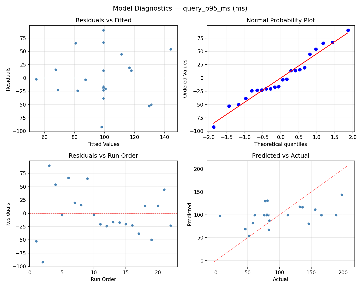
Response: query_p95_ms
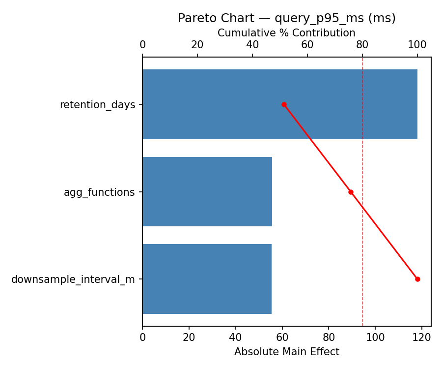
Top factors: retention_days (44.9%), downsample_interval_m (35.4%), agg_functions (19.7%).
ANOVA
| Source | DF | SS | MS | F | p-value |
|---|
| Source | DF | SS | MS | F | p-value |
| downsample_interval_m | 4 | 12737.6136 | 3184.4034 | 1.170 | 0.3857 |
| retention_days | 4 | 15310.9470 | 3827.7367 | 1.407 | 0.3070 |
| agg_functions | 4 | 10876.9470 | 2719.2367 | 1.000 | 0.4560 |
| Lack | of | Fit | 2 | 0.0000 | 0.0000 |
| Pure | Error | 7 | 19044.0000 | | |
| Error | 9 | 11490.8561 | 2720.5714 | | |
| Total | 21 | 50416.3636 | 2400.7792 | | |
Pareto Chart
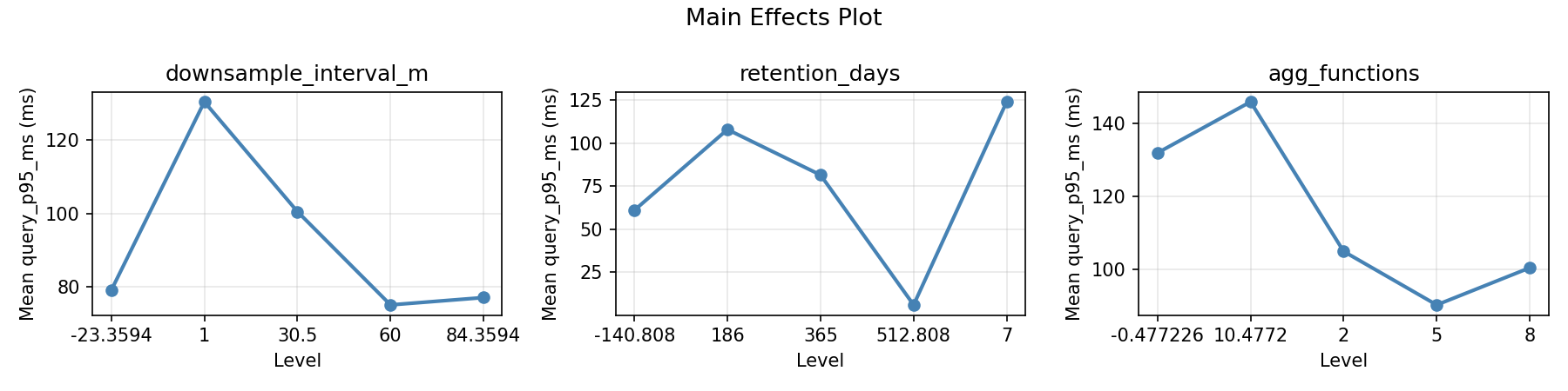
Main Effects Plot
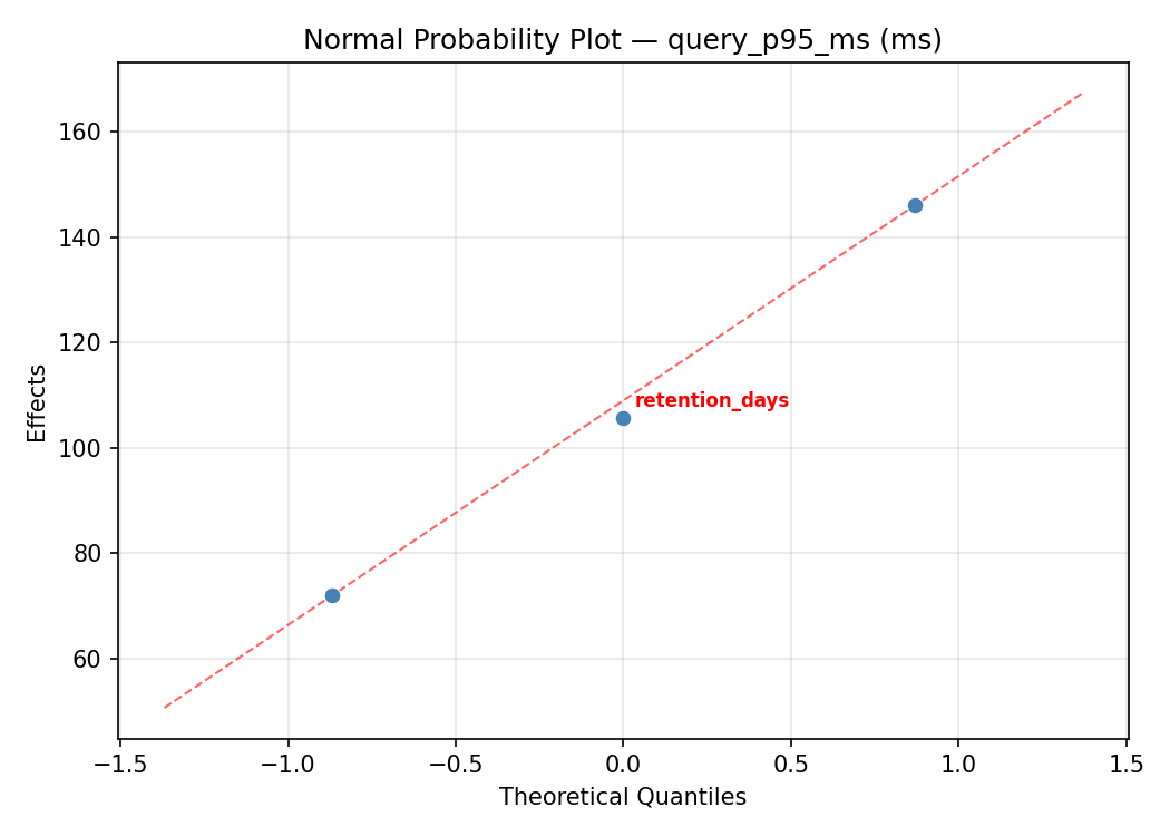
Normal Probability Plot of Effects
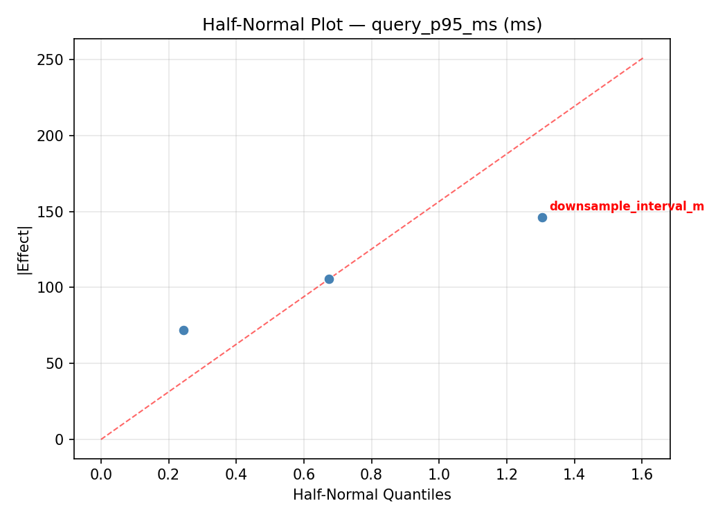
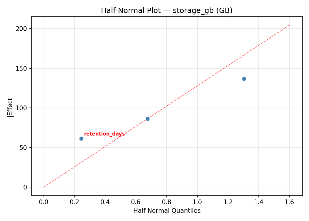
Half-Normal Plot of Effects
Model Diagnostics
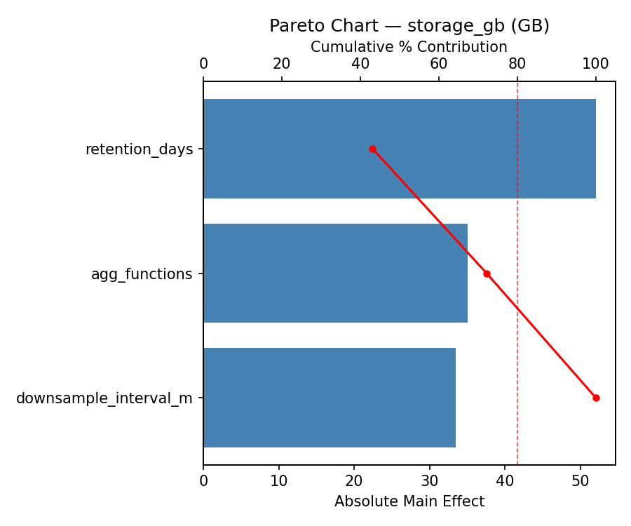
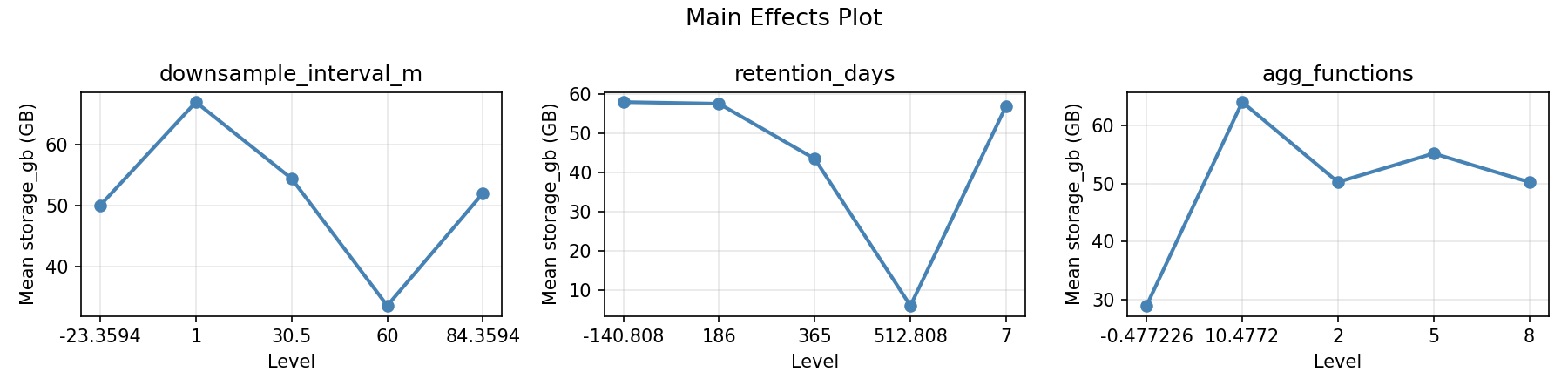
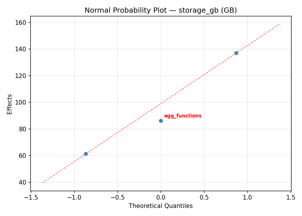
Response: storage_gb
Top factors: downsample_interval_m (43.6%), retention_days (34.8%), agg_functions (21.6%).
ANOVA
| Source | DF | SS | MS | F | p-value |
|---|
| Source | DF | SS | MS | F | p-value |
| downsample_interval_m | 4 | 6709.5682 | 1677.3920 | 1.027 | 0.4436 |
| retention_days | 4 | 5268.5682 | 1317.1420 | 0.807 | 0.5509 |
| agg_functions | 4 | 5661.9015 | 1415.4754 | 0.867 | 0.5194 |
| Lack | of | Fit | 2 | 0.0000 | 0.0000 |
| Pure | Error | 7 | 11427.5000 | | |
| Error | 9 | 8339.2803 | 1632.5000 | | |
| Total | 21 | 25979.3182 | 1237.1104 | | |
Pareto Chart
Main Effects Plot
Normal Probability Plot of Effects
Half-Normal Plot of Effects
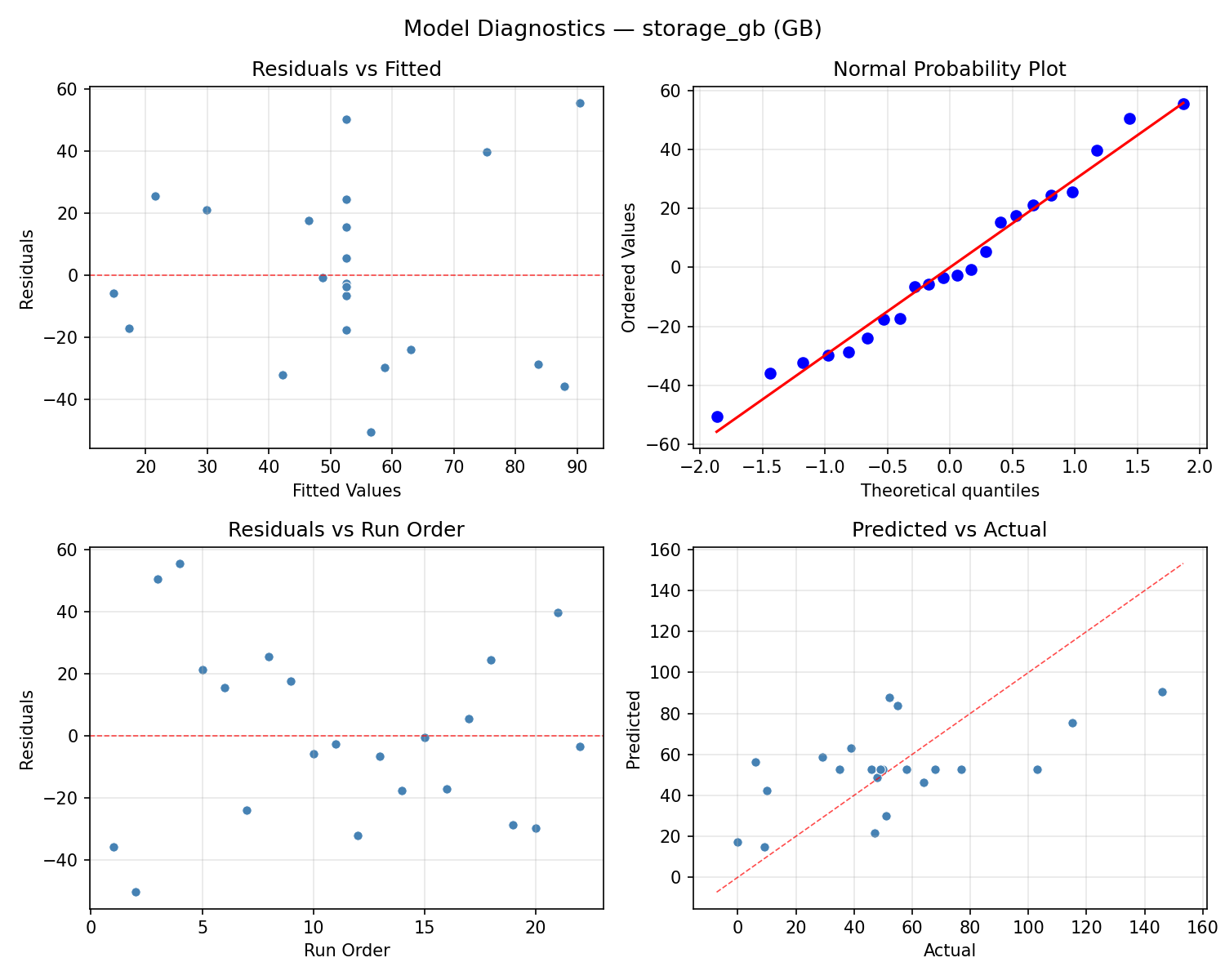
Model Diagnostics
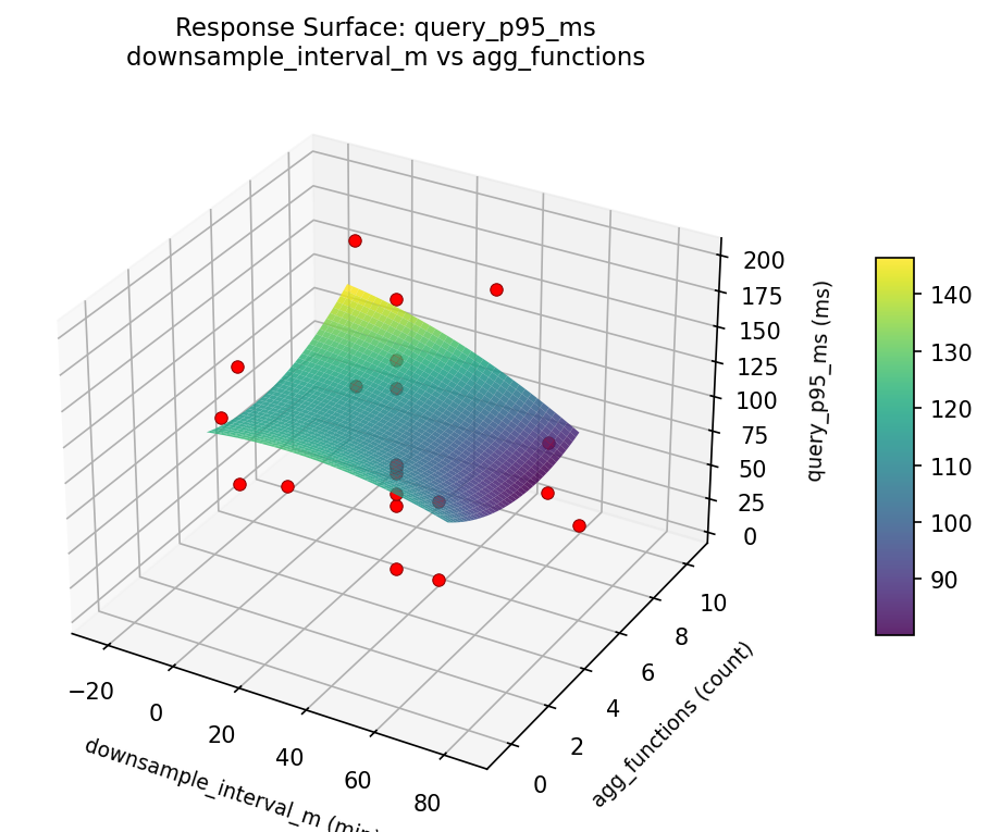
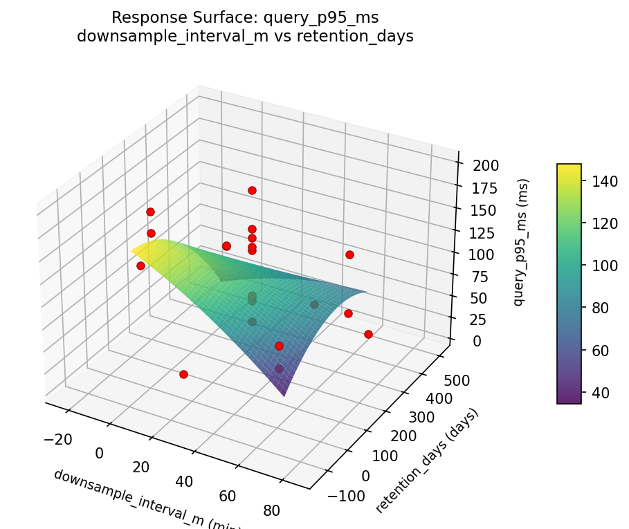
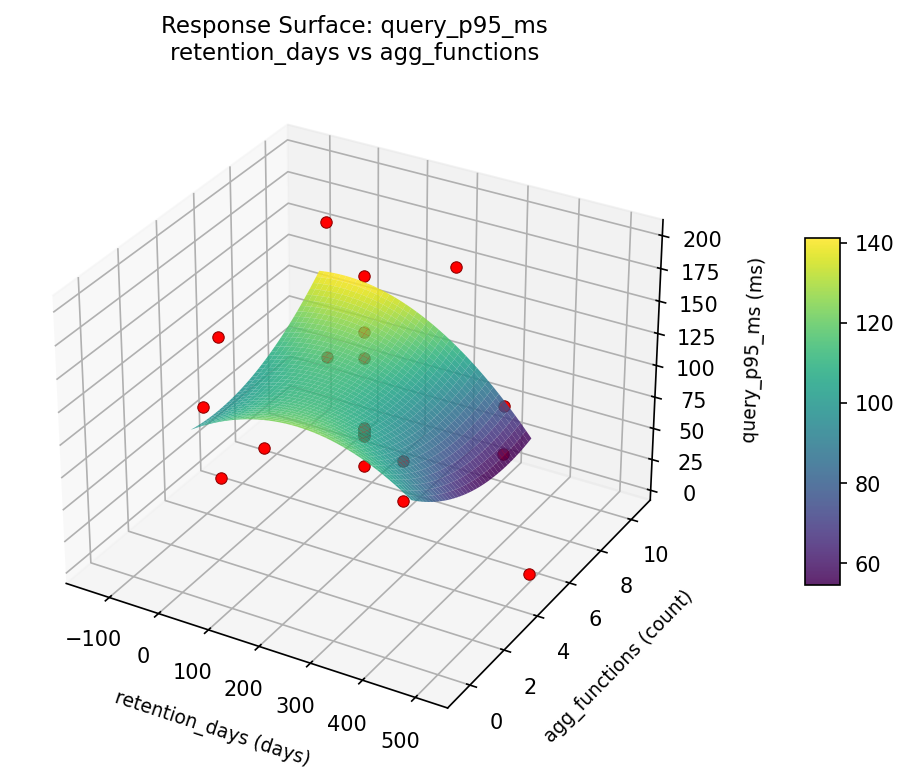
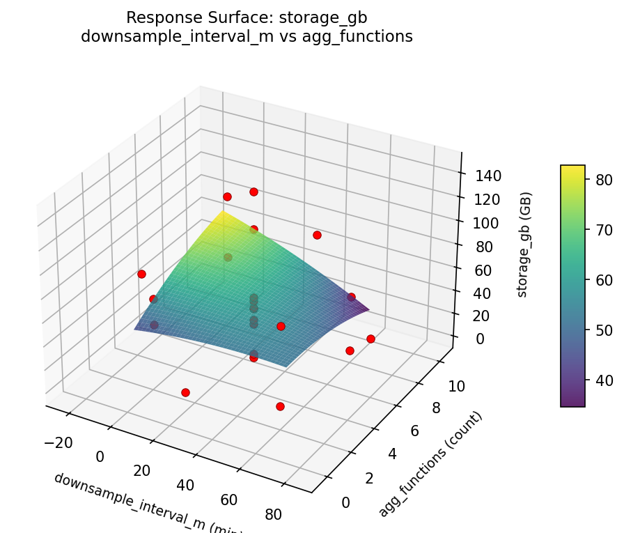
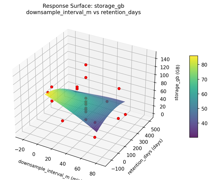
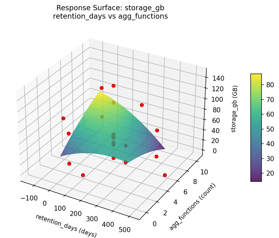
Response Surface Plots
3D surfaces fitted with quadratic RSM. Red dots are observed data points.
query p95 ms downsample interval m vs agg functions
query p95 ms downsample interval m vs retention days
query p95 ms retention days vs agg functions
storage gb downsample interval m vs agg functions
storage gb downsample interval m vs retention days
storage gb retention days vs agg functions
Multi-Objective Optimization
When responses compete, Derringer–Suich desirability finds the best compromise.
Each response is scaled to a 0–1 desirability, then combined via a weighted geometric mean.
Overall Desirability
D = 0.9394
Per-Response Desirability
| Response | Weight | Desirability | Predicted | Dir |
|---|
query_p95_ms |
1.5 |
|
6.00 0.9545 6.00 ms |
↓ |
storage_gb |
1.0 |
|
6.00 0.9172 6.00 GB |
↓ |
Recommended Settings
| Factor | Value |
|---|
downsample_interval_m | 1 min |
retention_days | 365 days |
agg_functions | 8 count |
Source: from observed run #2
Trade-off Summary
Sacrifice = how much worse than single-objective best.
| Response | Predicted | Best Observed | Sacrifice |
|---|
storage_gb | 6.00 | 0.00 | +6.00 |
Top 3 Runs by Desirability
| Run | D | Factor Settings |
|---|
| #16 | 0.8359 | downsample_interval_m=30.5, retention_days=186, agg_functions=5 |
| #10 | 0.7976 | downsample_interval_m=1, retention_days=7, agg_functions=8 |
Model Quality
| Response | R² | Type |
|---|
storage_gb | 0.4897 | linear |
Full Multi-Objective Output
============================================================
MULTI-OBJECTIVE OPTIMIZATION
Method: Derringer-Suich Desirability Function
============================================================
Overall desirability: D = 0.9394
Response Weight Desirability Predicted Direction
---------------------------------------------------------------------
query_p95_ms 1.5 0.9545 6.00 ms ↓
storage_gb 1.0 0.9172 6.00 GB ↓
Recommended settings:
downsample_interval_m = 1 min
retention_days = 365 days
agg_functions = 8 count
(from observed run #2)
Trade-off summary:
query_p95_ms: 6.00 (best observed: 6.00, sacrifice: +0.00)
storage_gb: 6.00 (best observed: 0.00, sacrifice: +6.00)
Model quality:
query_p95_ms: R² = 0.4343 (linear)
storage_gb: R² = 0.4897 (linear)
Top 3 observed runs by overall desirability:
1. Run #2 (D=0.9394): downsample_interval_m=1, retention_days=365, agg_functions=8
2. Run #16 (D=0.8359): downsample_interval_m=30.5, retention_days=186, agg_functions=5
3. Run #10 (D=0.7976): downsample_interval_m=1, retention_days=7, agg_functions=8
Full Analysis Output
=== Main Effects: query_p95_ms ===
Factor Effect Std Error % Contribution
--------------------------------------------------------------
retention_days 126.7500 10.4464 44.9%
downsample_interval_m 99.7500 10.4464 35.4%
agg_functions 55.6667 10.4464 19.7%
=== ANOVA Table: query_p95_ms ===
Source DF SS MS F p-value
-----------------------------------------------------------------------------
downsample_interval_m 4 12737.6136 3184.4034 1.170 0.3857
retention_days 4 15310.9470 3827.7367 1.407 0.3070
agg_functions 4 10876.9470 2719.2367 1.000 0.4560
Lack of Fit 2 0.0000 0.0000 0.000 1.0000
Pure Error 7 19044.0000 2720.5714
Error 9 11490.8561 2720.5714
Total 21 50416.3636 2400.7792
=== Summary Statistics: query_p95_ms ===
downsample_interval_m:
Level N Mean Std Min Max
------------------------------------------------------------
-23.3594 1 83.0000 0.0000 83.0000 83.0000
1 4 56.2500 36.6458 6.0000 84.0000
30.5 12 111.5000 50.4534 58.0000 198.0000
60 4 95.5000 43.3935 46.0000 146.0000
84.3594 1 156.0000 0.0000 156.0000 156.0000
retention_days:
Level N Mean Std Min Max
------------------------------------------------------------
-140.808 1 82.0000 0.0000 82.0000 82.0000
186 12 108.8333 46.5458 58.0000 198.0000
365 4 62.2500 46.4641 6.0000 113.0000
512.808 1 189.0000 0.0000 189.0000 189.0000
7 4 89.5000 39.9875 52.0000 146.0000
agg_functions:
Level N Mean Std Min Max
------------------------------------------------------------
-0.477226 1 80.0000 0.0000 80.0000 80.0000
10.4772 1 79.0000 0.0000 79.0000 79.0000
2 4 89.2500 16.1323 77.0000 113.0000
5 12 118.1667 50.6428 58.0000 198.0000
8 4 62.5000 59.2931 6.0000 146.0000
=== Main Effects: storage_gb ===
Factor Effect Std Error % Contribution
--------------------------------------------------------------
downsample_interval_m 87.0000 7.4988 43.6%
retention_days 69.5000 7.4988 34.8%
agg_functions 43.0833 7.4988 21.6%
=== ANOVA Table: storage_gb ===
Source DF SS MS F p-value
-----------------------------------------------------------------------------
downsample_interval_m 4 6709.5682 1677.3920 1.027 0.4436
retention_days 4 5268.5682 1317.1420 0.807 0.5509
agg_functions 4 5661.9015 1415.4754 0.867 0.5194
Lack of Fit 2 0.0000 0.0000 0.000 1.0000
Pure Error 7 11427.5000 1632.5000
Error 9 8339.2803 1632.5000
Total 21 25979.3182 1237.1104
=== Summary Statistics: storage_gb ===
downsample_interval_m:
Level N Mean Std Min Max
------------------------------------------------------------
-23.3594 1 47.0000 0.0000 47.0000 47.0000
1 4 28.0000 23.7908 6.0000 51.0000
30.5 12 57.5000 35.8722 10.0000 146.0000
60 4 48.2500 33.7478 0.0000 77.0000
84.3594 1 115.0000 0.0000 115.0000 115.0000
retention_days:
Level N Mean Std Min Max
------------------------------------------------------------
-140.808 1 35.0000 0.0000 35.0000 35.0000
186 12 59.5000 36.8622 10.0000 146.0000
365 4 33.5000 36.8646 0.0000 77.0000
512.808 1 103.0000 0.0000 103.0000 103.0000
7 4 42.7500 23.7118 9.0000 64.0000
agg_functions:
Level N Mean Std Min Max
------------------------------------------------------------
-0.477226 1 48.0000 0.0000 48.0000 48.0000
10.4772 1 50.0000 0.0000 50.0000 50.0000
2 4 56.5000 13.9164 46.0000 77.0000
5 12 62.8333 39.4089 10.0000 146.0000
8 4 19.7500 29.7363 0.0000 64.0000
Optimization Recommendations
=== Optimization: query_p95_ms ===
Direction: minimize
Best observed run: #2
downsample_interval_m = 1
retention_days = 365
agg_functions = 2
Value: 6.0
RSM Model (linear, R² = 0.1354, Adj R² = -0.0087):
Coefficients:
intercept +99.2727
downsample_interval_m +8.3063
retention_days -11.7205
agg_functions +16.0950
RSM Model (quadratic, R² = 0.4615, Adj R² = 0.0577):
Coefficients:
intercept +130.5885
downsample_interval_m +8.3063
retention_days -11.7205
agg_functions +16.0949
downsample_interval_m*retention_days +7.0000
downsample_interval_m*agg_functions -6.2500
retention_days*agg_functions -7.2500
downsample_interval_m^2 -17.7079
retention_days^2 -22.5079
agg_functions^2 -6.7579
Curvature analysis:
retention_days coef=-22.5079 concave (has a maximum)
downsample_interval_m coef=-17.7079 concave (has a maximum)
agg_functions coef=-6.7579 concave (has a maximum)
Notable interactions:
retention_days*agg_functions coef=-7.2500 (antagonistic)
downsample_interval_m*retention_days coef=+7.0000 (synergistic)
downsample_interval_m*agg_functions coef=-6.2500 (antagonistic)
Predicted optimum (from quadratic model, at observed points):
downsample_interval_m = 30.5
retention_days = 186
agg_functions = 10.4772
Predicted value: 137.4473
Surface optimum (via L-BFGS-B, quadratic model):
downsample_interval_m = 1
retention_days = 365
agg_functions = 2
Predicted value: 41.4931
Model quality: Weak fit — consider adding center points or using a different design.
Factor importance:
1. agg_functions (effect: 90.2, contribution: 41.1%)
2. retention_days (effect: 74.1, contribution: 33.7%)
3. downsample_interval_m (effect: 55.4, contribution: 25.2%)
=== Optimization: storage_gb ===
Direction: minimize
Best observed run: #16
downsample_interval_m = 30.5
retention_days = 512.808
agg_functions = 5
Value: 0.0
RSM Model (linear, R² = 0.0639, Adj R² = -0.0921):
Coefficients:
intercept +52.5909
downsample_interval_m +2.8192
retention_days -9.0965
agg_functions +4.7385
RSM Model (quadratic, R² = 0.3147, Adj R² = -0.1993):
Coefficients:
intercept +63.9725
downsample_interval_m +2.8192
retention_days -9.0965
agg_functions +4.7386
downsample_interval_m*retention_days +1.6250
downsample_interval_m*agg_functions -15.1250
retention_days*agg_functions +1.1250
downsample_interval_m^2 -6.8408
retention_days^2 -13.2908
agg_functions^2 +3.0592
Curvature analysis:
retention_days coef=-13.2908 concave (has a maximum)
downsample_interval_m coef=-6.8408 concave (has a maximum)
agg_functions coef=+3.0592 convex (has a minimum)
Notable interactions:
downsample_interval_m*agg_functions coef=-15.1250 (antagonistic)
downsample_interval_m*retention_days coef=+1.6250 (synergistic)
retention_days*agg_functions coef=+1.1250 (synergistic)
Predicted optimum (from linear model, at observed points):
downsample_interval_m = 60
retention_days = 7
agg_functions = 8
Predicted value: 69.2452
Surface optimum (via L-BFGS-B, linear model):
downsample_interval_m = 1
retention_days = 365
agg_functions = 2
Predicted value: 35.9366
Model quality: Weak fit — consider adding center points or using a different design.
Factor importance:
1. agg_functions (effect: 81.0, contribution: 47.0%)
2. retention_days (effect: 64.9, contribution: 37.6%)
3. downsample_interval_m (effect: 26.6, contribution: 15.4%)