Summary
This experiment investigates ml hyperparameter screening. Fractional factorial to screen 5 hyperparameters with minimal runs.
The design varies 5 factors: learning rate, ranging from 0.001 to 0.1, batch size, ranging from 32 to 256, dropout, ranging from 0.1 to 0.5, hidden layers, ranging from 2 to 6, and optimizer, ranging from sgd to adam. The goal is to optimize 2 responses: accuracy (%) (maximize) and training time (sec) (minimize). Fixed conditions held constant across all runs include epochs = 50, dataset = cifar10.
A fractional factorial design reduces the number of runs from 32 to 8 by deliberately confounding higher-order interactions. This is ideal for screening — identifying which of the 5 factors matter most before investing in a full study.
Key Findings
For accuracy, the most influential factors were learning rate (34.8%), dropout (32.5%), batch size (22.6%). The best observed value was 78.1 (at learning rate = 0.001, batch size = 256, dropout = 0.1).
For training time, the most influential factors were learning rate (33.2%), dropout (29.0%), batch size (23.3%). The best observed value was 77.3 (at learning rate = 0.001, batch size = 256, dropout = 0.1).
Recommended Next Steps
- Follow up with a response surface design (CCD or Box-Behnken) on the top 3–4 factors to model curvature and find the true optimum.
- Consider whether any fixed factors should be varied in a future study.
- The screening results can guide factor reduction — drop factors contributing less than 5% and re-run with a smaller, more focused design.
The Scenario
You are training a deep learning model and need to screen 5 hyperparameters to find which ones matter most. A full factorial would require 25 = 32 runs, and each training run takes significant GPU time. A fractional factorial cuts this in half.
Why Fractional Factorial?
Resolution III fractional factorial uses only 16 runs. You're screening — you just need to know which hyperparameters have the largest effects. Some main effects are aliased with 2-factor interactions, but follow-up experiments can resolve ambiguities.
Experimental Setup
Factors
| Factor | Low | High | Type |
|---|---|---|---|
learning_rate | 0.001 | 0.1 | continuous |
batch_size | 32 | 256 | continuous |
dropout | 0.1 | 0.5 | continuous |
hidden_layers | 2 | 6 | continuous |
optimizer | sgd | adam | categorical |
Fixed: epochs = 50, dataset = cifar10
Responses
| Response | Direction | Unit |
|---|---|---|
accuracy | ↑ maximize | % |
training_time | ↓ minimize | sec |
Conflicting objectives
Look for factors that improve accuracy without hurting training time — those are the "free wins."
Experimental Matrix
The Fractional Factorial Design produces 8 runs. Each row is one experiment with specific factor settings.
| Run | learning_rate | batch_size | dropout | hidden_layers | optimizer |
|---|---|---|---|---|---|
| 1 | 0.001 | 256 | 0.5 | 2 | sgd |
| 2 | 0.1 | 32 | 0.1 | 2 | sgd |
| 3 | 0.1 | 256 | 0.1 | 6 | sgd |
| 4 | 0.1 | 256 | 0.5 | 6 | adam |
| 5 | 0.001 | 256 | 0.1 | 2 | adam |
| 6 | 0.1 | 32 | 0.5 | 2 | adam |
| 7 | 0.001 | 32 | 0.1 | 6 | adam |
| 8 | 0.001 | 32 | 0.5 | 6 | sgd |
Step-by-Step Workflow
Positional argument style
This use case uses positional args: factors are passed in order without flag names. The runner script calls sim.sh 0.001 32 0.1 2 sgd --out run_1.json. Useful when your training script expects ordered arguments.
Features Exercised
| Feature | Value |
|---|---|
| Design type | fractional_factorial |
| Factor types | continuous (4) + categorical (1) |
| Arg style | positional |
| Run reduction | 16 runs instead of 32 (50% savings) |
| Multi-response | accuracy ↑, training_time ↓ |
--seed | 7 (reproducible run order) |
Analysis Results
Generated from actual experiment runs using the DOE Helper Tool.
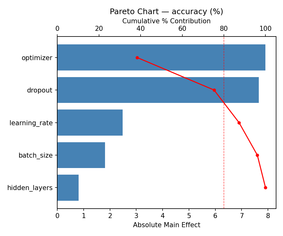
Response: accuracy
The Pareto chart identifies which hyperparameters contribute most to model accuracy.
Pareto Chart
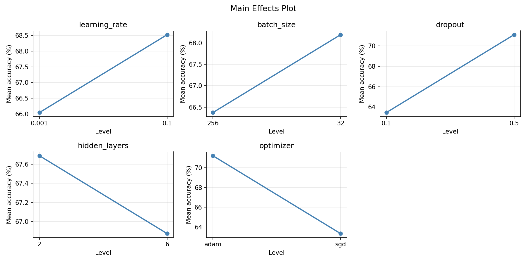
Main Effects Plot
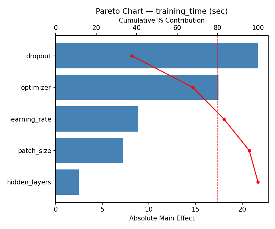
Response: training_time
Training time is driven by a different set of hyperparameters, revealing trade-offs with accuracy.
Pareto Chart
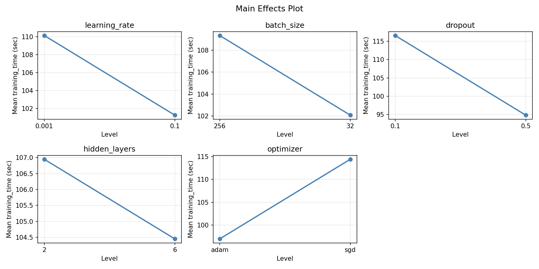
Main Effects Plot
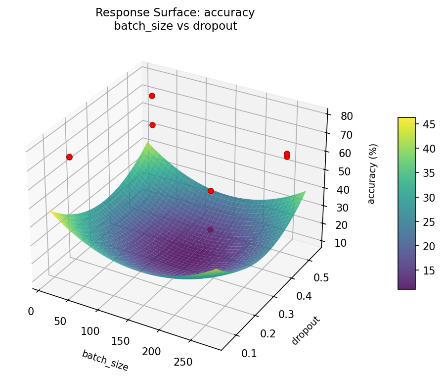
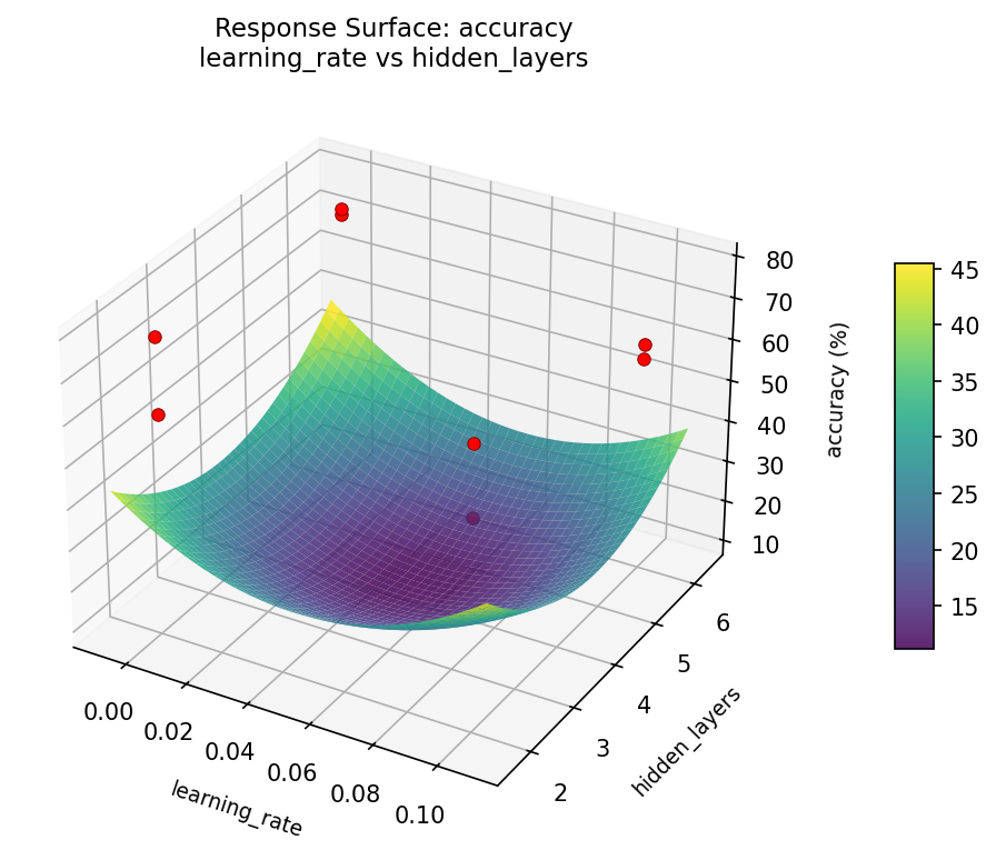
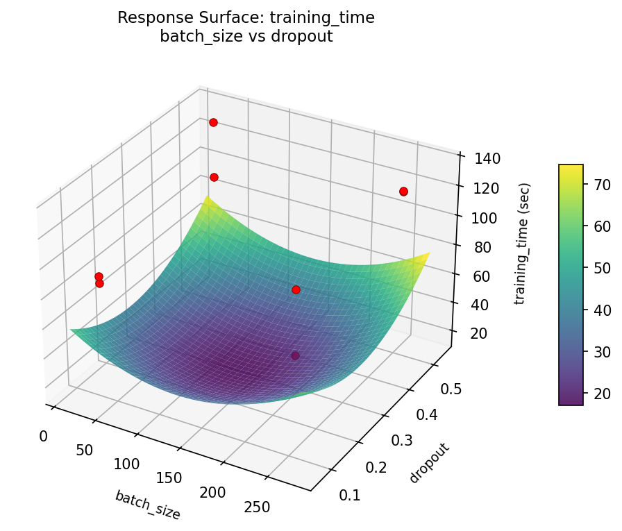
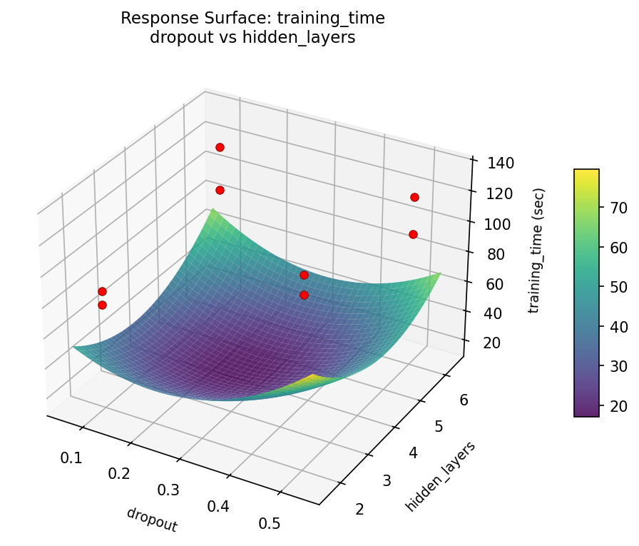
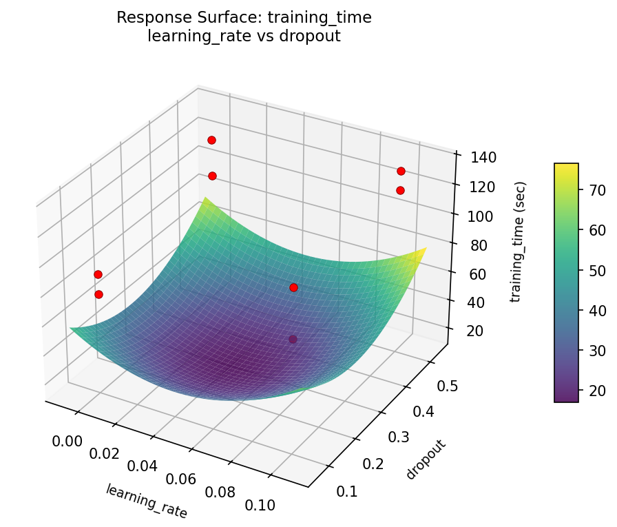
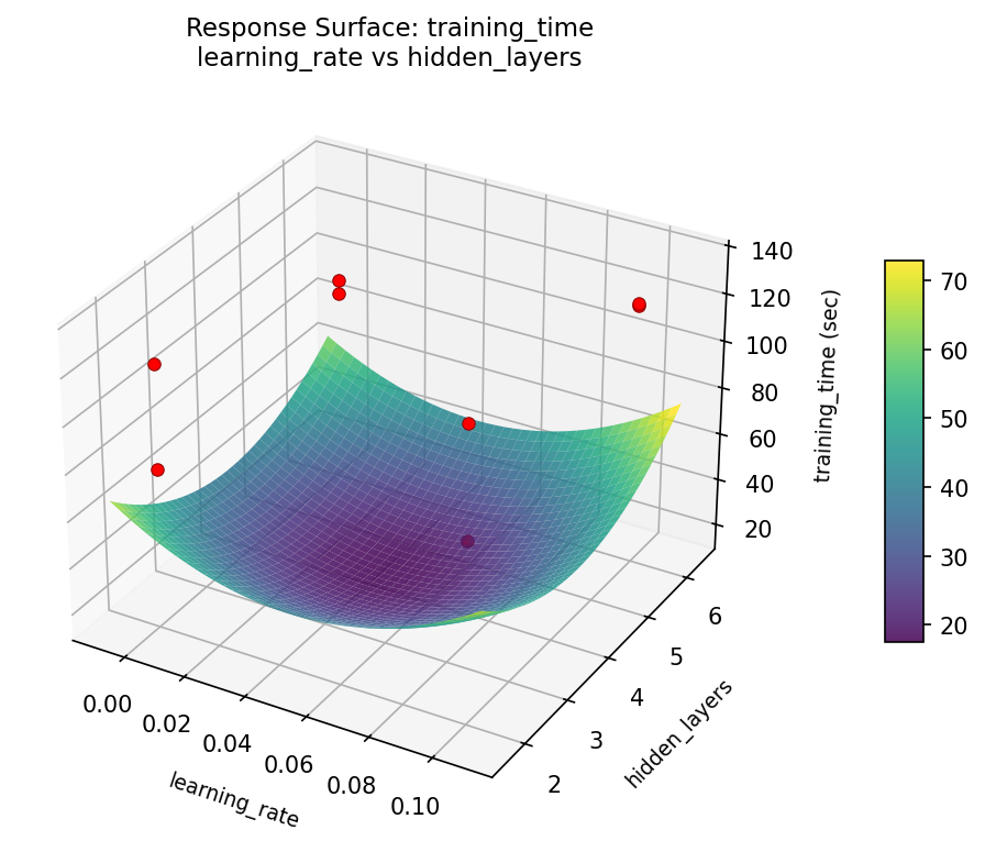
Response Surface Plots
3D surfaces fitted with quadratic RSM. Red dots are observed data points.
How to Read These Surfaces
Each plot shows predicted response (vertical axis) across two factors while other factors are held at center. Red dots are actual experimental observations.
- Flat surface — these two factors have little effect on the response.
- Tilted plane — strong linear effect; moving along one axis consistently changes the response.
- Curved/domed surface — quadratic curvature; there is an optimum somewhere in the middle.
- Saddle shape — significant interaction; the best setting of one factor depends on the other.
- Red dots far from surface — poor model fit in that region; be cautious about predictions there.
accuracy (%) — R² = 1.000, Adj R² = 1.000
The model fits well — the surface shape is reliable.
Curvature detected in learning_rate, batch_size — look for a peak or valley in the surface.
Strongest linear driver: batch_size (decreases accuracy).
Notable interaction: learning_rate × hidden_layers — the effect of one depends on the level of the other. Look for a twisted surface.
training_time (sec) — R² = 1.000, Adj R² = 1.000
The model fits well — the surface shape is reliable.
Curvature detected in learning_rate, batch_size — look for a peak or valley in the surface.
Strongest linear driver: batch_size (increases training_time).
Notable interaction: learning_rate × hidden_layers — the effect of one depends on the level of the other. Look for a twisted surface.
accuracy: batch size vs dropout
accuracy: batch size vs hidden layers

accuracy: dropout vs hidden layers

accuracy: learning rate vs batch size

accuracy: learning rate vs dropout

accuracy: learning rate vs hidden layers
training: time batch size vs dropout
training: time batch size vs hidden layers

training: time dropout vs hidden layers
training: time learning rate vs batch size

training: time learning rate vs dropout
training: time learning rate vs hidden layers
Full Analysis Output
Optimization Recommendations
Multi-Objective Optimization
When responses compete, Derringer–Suich desirability finds the best compromise. Each response is scaled to a 0–1 desirability, then combined via a weighted geometric mean.
Per-Response Desirability
| Response | Weight | Desirability | Predicted | Dir |
|---|---|---|---|---|
accuracy |
1.5 |
1.0000
|
80.87 1.0000 80.87 % | ↑ |
training_time |
1.0 |
1.0000
|
73.29 1.0000 73.29 sec | ↓ |
Recommended Settings
| Factor | Value |
|---|---|
learning_rate | 0.09247 |
batch_size | 34.55 |
dropout | 0.4207 |
hidden_layers | 5.91 |
optimizer | adam |
Source: from RSM model prediction
Trade-off Summary
Sacrifice = how much worse than single-objective best.
| Response | Predicted | Best Observed | Sacrifice |
|---|---|---|---|
training_time | 73.29 | 77.30 | -4.01 |
Top 3 Runs by Desirability
| Run | D | Factor Settings |
|---|---|---|
| #3 | 0.8029 | learning_rate=0.1, batch_size=256, dropout=0.5, hidden_layers=6, optimizer=adam |
| #6 | 0.7830 | learning_rate=0.001, batch_size=32, dropout=0.5, hidden_layers=6, optimizer=sgd |
Model Quality
| Response | R² | Type |
|---|---|---|
training_time | 0.9277 | linear |