Summary
This experiment investigates distillation column optimization. Central Composite Design to model and optimize separation efficiency.
The design varies 3 factors: reflux ratio, ranging from 1.5 to 4.5, feed rate (L/h), ranging from 50 to 150, and column pressure (atm), ranging from 1.0 to 3.0. The goal is to optimize 2 responses: separation efficiency (%) (maximize) and energy cost (USD/h) (minimize). Fixed conditions held constant across all runs include feed temp = 80, n trays = 20.
A Central Composite Design (CCD) was selected to fit a full quadratic response surface model, including curvature and interaction effects. With 3 factors this produces 22 runs including center points and axial (star) points that extend beyond the factorial range.
Quadratic response surface models were fitted to capture potential curvature and factor interactions. The RSM contour plots below visualize how pairs of factors jointly affect each response.
Key Findings
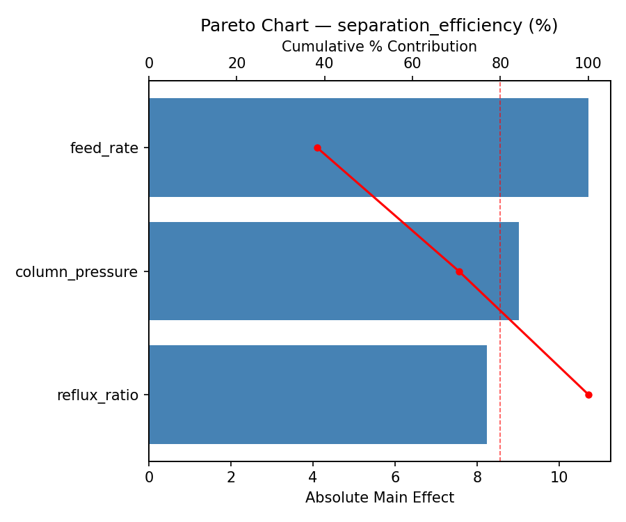
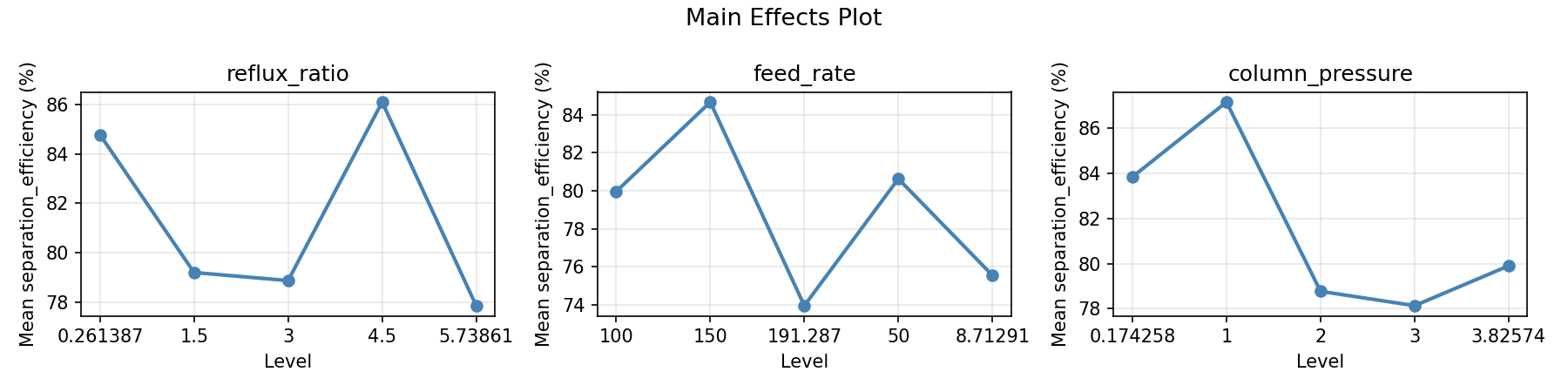
For separation efficiency, the most influential factors were feed rate (39.9%), reflux ratio (30.2%), column pressure (29.9%). The best observed value was 91.68 (at reflux ratio = 3, feed rate = 100, column pressure = 2).
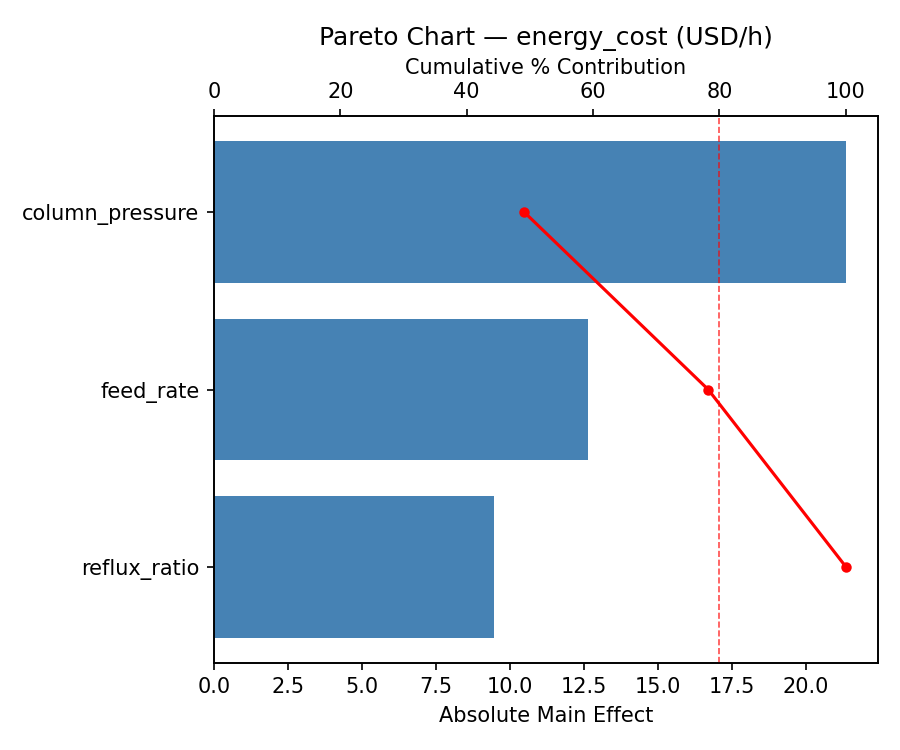
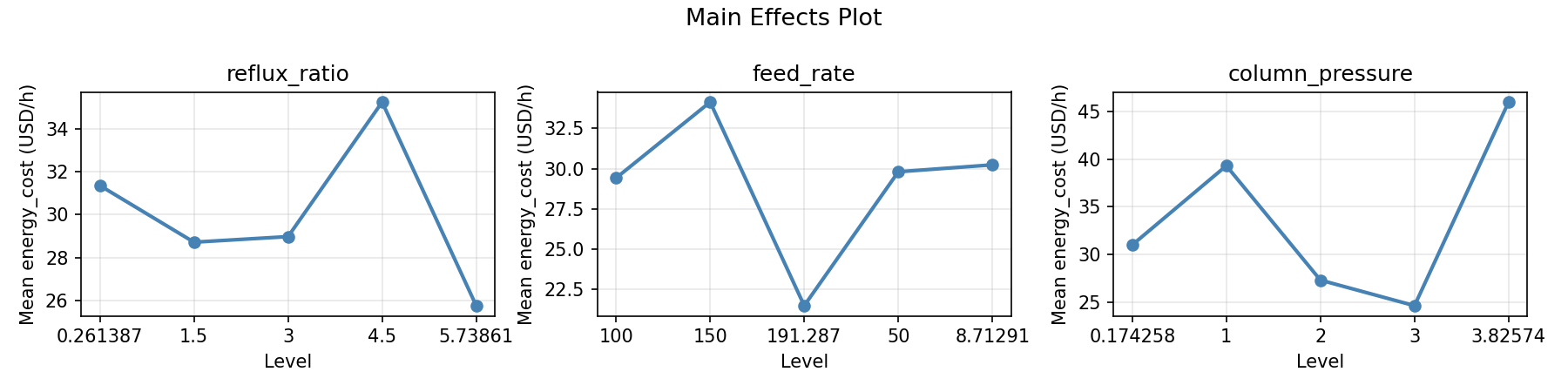
For energy cost, the most influential factors were feed rate (43.9%), column pressure (41.8%), reflux ratio (14.3%). The best observed value was 10.03 (at reflux ratio = 1.5, feed rate = 150, column pressure = 1).
Recommended Next Steps
- Run confirmation experiments at the predicted optimal settings to validate the model.
- Consider whether any fixed factors should be varied in a future study.
The Scenario
You are optimizing a distillation column for maximum separation efficiency at minimum energy cost. You suspect the response surface is curved (quadratic), so you need a design with star points and center points to fit a second-order model.
Why Central Composite Design?
CCD = factorial (23=8) + star (2×3=6) + center (8) = 22 runs. Star points at ±α extend beyond the factorial cube to probe curvature. Center replicates estimate pure error. Orthogonal alpha ensures balanced estimation of all model terms.
Experimental Setup
Factors
| Factor | Low | High | Unit |
|---|---|---|---|
reflux_ratio | 1.5 | 4.5 | L/D |
feed_rate | 50 | 150 | L/h |
column_pressure | 1.0 | 3.0 | atm |
Fixed: feed_temp = 80°C, n_trays = 20
Responses
| Response | Direction | Unit |
|---|---|---|
separation_efficiency | ↑ maximize | % |
energy_cost | ↓ minimize | USD/h |
CCD Run Structure
Experimental Matrix
The Central Composite Design produces 22 runs. Each row is one experiment with specific factor settings.
| Run | reflux_ratio | feed_rate | column_pressure |
|---|---|---|---|
| 1 | 3 | 100 | 2 |
| 2 | 4.5 | 50 | 3 |
| 3 | 1.5 | 150 | 1 |
| 4 | 3 | 191.287 | 2 |
| 5 | 3 | 100 | 2 |
| 6 | 0.261387 | 100 | 2 |
| 7 | 3 | 100 | 0.174258 |
| 8 | 3 | 100 | 2 |
| 9 | 4.5 | 150 | 1 |
| 10 | 5.73861 | 100 | 2 |
| 11 | 3 | 100 | 2 |
| 12 | 3 | 8.71291 | 2 |
| 13 | 3 | 100 | 2 |
| 14 | 1.5 | 50 | 3 |
| 15 | 3 | 100 | 2 |
| 16 | 4.5 | 50 | 1 |
| 17 | 3 | 100 | 3.82574 |
| 18 | 4.5 | 150 | 3 |
| 19 | 3 | 100 | 2 |
| 20 | 1.5 | 50 | 1 |
| 21 | 1.5 | 150 | 3 |
| 22 | 3 | 100 | 2 |
Step-by-Step Workflow
This use case demonstrates the full pipeline — every command the tool offers:
Star points extend beyond [low, high]
Some runs have factor values outside the [low, high] range (e.g., reflux_ratio below 1.5 or above 4.5). This is the CCD's circumscribed design: the factorial cube is inscribed within the star points. Make sure your equipment can handle these extended ranges.
Real-World Plant Workflow
Running on Real Equipment? Use the Manual Workflow
Distillation column optimization involves adjusting physical equipment — reflux valves, reboiler temperature, feed rates — and taking samples for analysis. Each run may take hours to reach steady state. The simulation above is for demonstration; for real plant trials, use the manual workflow.
Plant experiments often run one or two conditions per shift. Here's how to manage the process:
Built for Multi-Day Experiments
Distillation trials often span multiple shifts or days. The status command tracks progress across sessions, record saves results one at a time as each steady-state condition is reached, and --partial analysis lets the process engineer evaluate trends before all conditions have been tested — critical when plant time is expensive.
Interpreting the Results
Trade-offs
- Higher reflux ratio → better separation but much higher energy cost
- Higher feed rate → moderate effect on both responses
- Higher pressure → improves separation with moderate energy increase
Single vs. Multi-Response Optimization
The --response flag
Compare optimize --response separation_efficiency (ignores cost) vs. optimize (all responses). The settings that maximize efficiency often increase energy cost. This reveals the Pareto frontier — the set of optimal trade-offs.
Next Steps
- Fit a full quadratic RSM model using the CCD data
- Construct a desirability function weighting efficiency vs. cost
- Find the Pareto-optimal frontier
- Run confirmation experiments at the predicted optimum
Features Exercised
| Feature | Value |
|---|---|
| Design type | central_composite (circumscribed, orthogonal α) |
| Factor types | continuous (all 3) |
| Star points | Yes (extends beyond [low, high]) |
| Center replicates | 8 center points for error estimation |
--response | Single-response optimization |
--csv | Export for custom modeling |
| Full pipeline | info → generate → run → analyze → optimize → report → csv |
| Total runs | 22 (8 factorial + 6 star + 8 center) |
Analysis Results
Generated from actual experiment runs using the DOE Helper Tool.
Response: separation_efficiency
The Pareto chart identifies which column parameters most strongly influence separation efficiency.
Pareto Chart
Main Effects Plot
Response: energy_cost
Energy cost responds to a different set of column parameters, requiring careful optimization against separation efficiency.
Pareto Chart
Main Effects Plot
Response Surface Plots
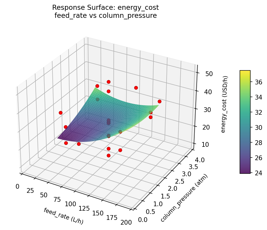
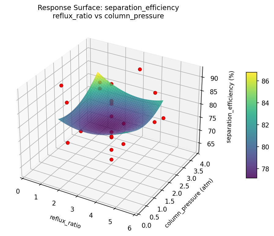
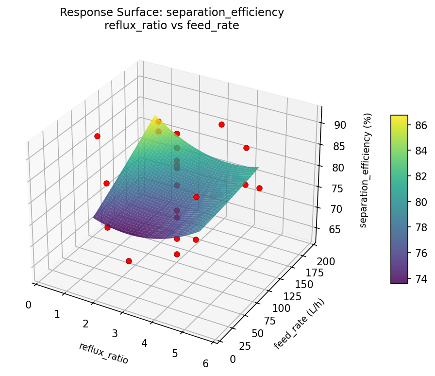
3D surfaces fitted with quadratic RSM. Red dots are observed data points.
How to Read These Surfaces
Each plot shows predicted response (vertical axis) across two factors while other factors are held at center. Red dots are actual experimental observations.
- Flat surface — these two factors have little effect on the response.
- Tilted plane — strong linear effect; moving along one axis consistently changes the response.
- Curved/domed surface — quadratic curvature; there is an optimum somewhere in the middle.
- Saddle shape — significant interaction; the best setting of one factor depends on the other.
- Red dots far from surface — poor model fit in that region; be cautious about predictions there.
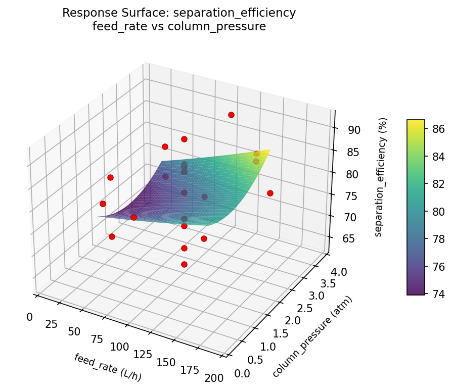
separation_efficiency (%) — R² = 0.312, Adj R² = -0.204
Weak fit — interpret the surface shape with caution.
Curvature detected in reflux_ratio, column_pressure — look for a peak or valley in the surface.
Strongest linear driver: column_pressure (decreases separation_efficiency).
Notable interaction: reflux_ratio × feed_rate — the effect of one depends on the level of the other. Look for a twisted surface.
energy_cost (USD/h) — R² = 0.277, Adj R² = -0.265
Weak fit — interpret the surface shape with caution.
Curvature detected in column_pressure, reflux_ratio — look for a peak or valley in the surface.
Strongest linear driver: reflux_ratio (decreases energy_cost).
Notable interaction: reflux_ratio × feed_rate — the effect of one depends on the level of the other. Look for a twisted surface.
energy: cost feed rate vs column pressure
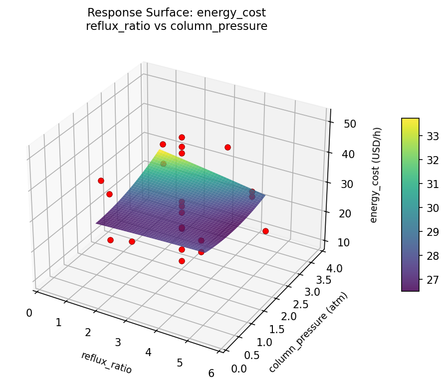
energy: cost reflux ratio vs column pressure
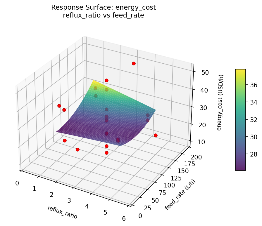
energy: cost reflux ratio vs feed rate
separation: efficiency feed rate vs column pressure
separation: efficiency reflux ratio vs column pressure
separation: efficiency reflux ratio vs feed rate
Full Analysis Output
Optimization Recommendations
Multi-Objective Optimization
When responses compete, Derringer–Suich desirability finds the best compromise. Each response is scaled to a 0–1 desirability, then combined via a weighted geometric mean.
Per-Response Desirability
| Response | Weight | Desirability | Predicted | Dir |
|---|---|---|---|---|
separation_efficiency |
2.0 |
0.7855
|
86.42 0.7855 86.42 % | ↑ |
energy_cost |
1.0 |
0.5426
|
28.63 0.5426 28.63 USD/h | ↓ |
Recommended Settings
| Factor | Value |
|---|---|
reflux_ratio | 4.5 |
feed_rate | 150 L/h |
column_pressure | 1 atm |
Source: from observed run #5
Trade-off Summary
Sacrifice = how much worse than single-objective best.
| Response | Predicted | Best Observed | Sacrifice |
|---|---|---|---|
energy_cost | 28.63 | 10.03 | +18.60 |
Top 3 Runs by Desirability
| Run | D | Factor Settings |
|---|---|---|
| #19 | 0.6819 | reflux_ratio=3, feed_rate=100, column_pressure=2 |
| #15 | 0.6783 | reflux_ratio=3, feed_rate=100, column_pressure=2 |
Model Quality
| Response | R² | Type |
|---|---|---|
energy_cost | 0.0694 | linear |