Material Formulation — DOE Use Case

Summary

This experiment investigates composite material formulation. Latin Hypercube sampling to explore a 4-factor material design space.

The design varies 4 factors: polymer ratio, ranging from 0.3 to 0.8, filler pct (%), ranging from 5 to 30, cure temp (C), ranging from 120 to 200, and particle size, ranging from fine to coarse. The goal is to optimize 2 responses: tensile strength (MPa) (maximize) and flexibility (mm) (maximize). Fixed conditions held constant across all runs include cure time min = 45, ambient humidity = 50.

Latin Hypercube Sampling was used to space 20 runs across the 4-dimensional factor space with good coverage and minimal gaps, making it ideal for computer experiments where the response surface may be complex.

Quadratic response surface models were fitted to capture potential curvature and factor interactions. The RSM contour plots below visualize how pairs of factors jointly affect each response.

Key Findings

For tensile strength, the most influential factors were polymer ratio (31.9%), filler pct (31.9%), cure temp (31.9%). The best observed value was 65.8 (at polymer ratio = 0.407722, filler pct = 16.2091, cure temp = 190.393).

For flexibility, the most influential factors were polymer ratio (30.7%), filler pct (30.7%), cure temp (30.7%). The best observed value was 15.14 (at polymer ratio = 0.332938, filler pct = 21.6368, cure temp = 182.028).

Recommended Next Steps

Consider whether any fixed factors should be varied in a future study.

The Scenario

You are developing a new composite material and need to explore a large, continuous design space. With 4 factors (3 continuous + 1 ordinal), you want good coverage without testing every combination. Latin Hypercube Sampling gives you space-filling coverage that captures the full range of each factor.

ℹ

Why Latin Hypercube?

Continuous factors need interpolation, not just high/low. LHS divides each factor's range into N equal intervals and places exactly one sample in each interval — like placing non-attacking rooks on a chessboard. The maximin criterion ensures no clustering. With lhs_samples: 20, you get double the default coverage.

Experimental Setup

Factors

Factor	Range / Levels	Type	Unit
`polymer_ratio`	0.3 – 0.8	continuous	—
`filler_pct`	5 – 30	continuous	%
`cure_temp`	120 – 200	continuous	°C
`particle_size`	fine, medium, coarse	ordinal	—

Fixed: cure_time = 45 min, ambient_humidity = 50%

Responses

Response	Direction	Unit
`tensile_strength`	↑ maximize	MPa
`flexibility`	↑ maximize	mm

Experimental Matrix

The Latin Hypercube Design produces 20 runs. Each row is one experiment with specific factor settings.

Run	`polymer_ratio`	`filler_pct`	`cure_temp`	`particle_size`
1	0.566054	21.6859	134.959	medium
2	0.367783	5.37721	182.616	coarse
3	0.496529	29.9263	145.802	medium
4	0.778077	27.4259	159.904	fine
5	0.457949	9.69109	129.737	fine
6	0.52125	6.33153	164.164	fine
7	0.658168	18.7417	177.008	medium
8	0.63707	11.5863	154.58	coarse
9	0.435564	13.7306	148.935	coarse
10	0.739761	19.9688	126.452	fine
11	0.534888	23.1088	168.658	coarse
12	0.331599	8.23897	141.403	fine
13	0.593778	17.2912	195.577	fine
14	0.310305	10.5245	172.294	medium
15	0.691865	13.7707	199.302	medium
16	0.718113	24.6354	186.151	medium
17	0.385691	25.3553	121.335	medium
18	0.62317	28.6331	161.748	fine
19	0.77194	20.4604	190.753	coarse
20	0.417421	16.1789	138.561	coarse

Step-by-Step Workflow

Complete workflow

# Preview: 20 LHS samples (custom, not default 10)
$ doe info --config use_cases/05_material_formulation/config.json

# Generate with seed for reproducible LHS sampling
$ doe generate --config use_cases/05_material_formulation/config.json \
    --output results/run.sh --seed 99

# Execute
$ bash results/run.sh

# Analyze with --results-dir override
$ doe analyze --config use_cases/05_material_formulation/config.json \
    --results-dir use_cases/05_material_formulation/results

# Optimize and report
$ doe optimize --config use_cases/05_material_formulation/config.json
$ doe report --config use_cases/05_material_formulation/config.json \
    --output results/report.html

Real-World Lab Workflow

ℹ

Physical Material Testing? Use the Manual Workflow

Composite material formulation is inherently physical — you mix resins, prepare specimens, cure them, and run tensile tests on a universal testing machine. The simulation script above is for demonstration. In practice, use record, status, and export-worksheet for your real experiments.

Material testing typically spans days (due to curing times) and involves expensive specimens. Here's the practical workflow:

Manual workflow for material testing

# 1. Print a worksheet for the lab
$ doe export-worksheet --config use_cases/05_material_formulation/config.json \
    --format csv --output formulation_worksheet.csv

# 2. Check which specimens to prepare next
$ doe status --config use_cases/05_material_formulation/config.json

# 3. After testing each specimen, record the results
$ doe record --config use_cases/05_material_formulation/config.json --run 1
# Enter tensile_strength, elongation, etc. when prompted

# 4. Peek at results after half the specimens are tested
$ doe analyze --config use_cases/05_material_formulation/config.json --partial

# 5. Full analysis when all specimens are done
$ doe analyze --config use_cases/05_material_formulation/config.json
$ doe optimize --config use_cases/05_material_formulation/config.json
$ doe report --config use_cases/05_material_formulation/config.json \
    --output formulation_report.html

✔

Ideal for Expensive Experiments

Material specimens can be costly and slow to prepare. The --partial flag lets you analyze intermediate results — if one factor clearly dominates after half the specimens, you can make informed decisions about whether to continue, adjust, or pivot the study before committing more materials.

Interpreting the Results

Continuous Factor Coverage

Unlike 2-level designs where each factor takes only "low" or "high," LHS produces unique values across the entire range. This enables:

Detecting non-linear effects (e.g., cure_temp has a quadratic effect on tensile strength)
Building regression models with better interpolation
Identifying narrow optimal regions within the factor space

Ordinal Factor Handling

The ordinal factor particle_size is binned into its 3 levels (fine, medium, coarse). About 1/3 of the 20 runs use each level, spread across the LHS sample.

Next Steps

Identify the most promising region from LHS results
Narrow the factor ranges around that region
Run a Box-Behnken or CCD for precise optimization

Features Exercised

Feature	Value
Design type	`latin_hypercube`
Factor types	`continuous` (3) + `ordinal` (1, 3 levels)
`lhs_samples`	20 (custom, overrides default of 10)
`--results-dir`	Override at analysis time
`--seed`	99 (controls numpy RNG for LHS)
Multi-response	tensile_strength ↑, flexibility ↑

Analysis Results

Generated from actual experiment runs using the DOE Helper Tool.

Response: tensile_strength

The Pareto chart reveals which formulation components most strongly affect tensile strength.

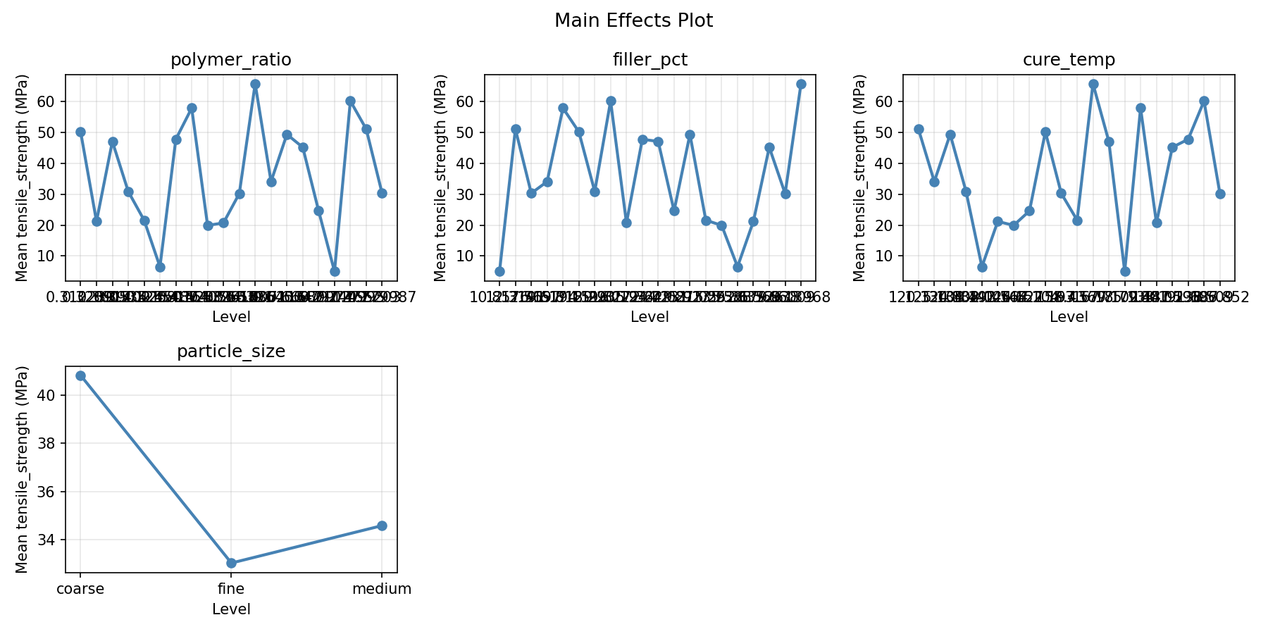
Pareto Chart

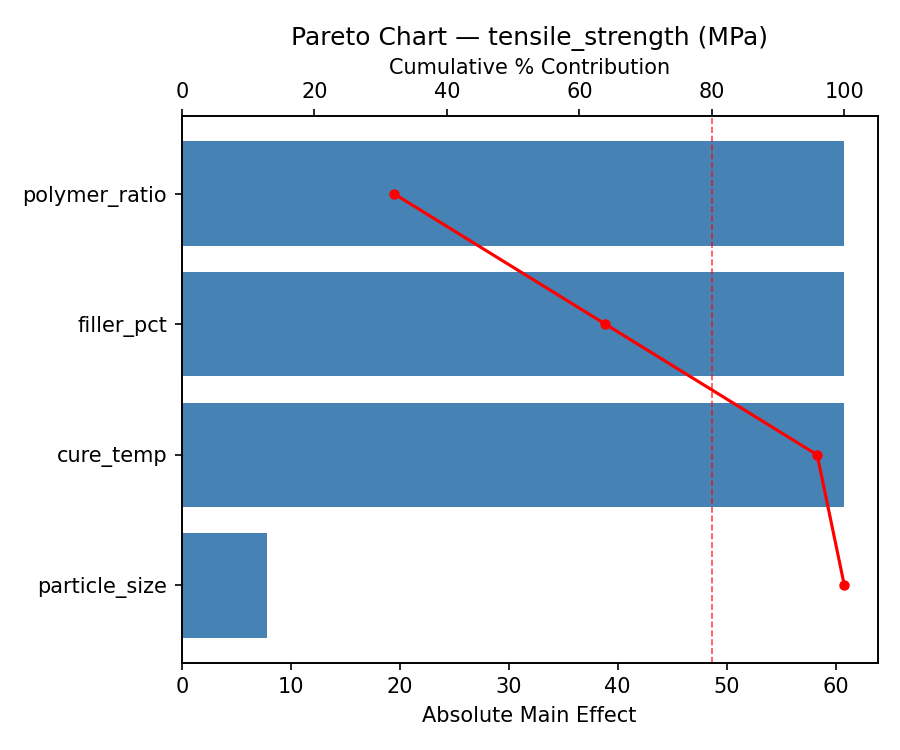
Main Effects Plot

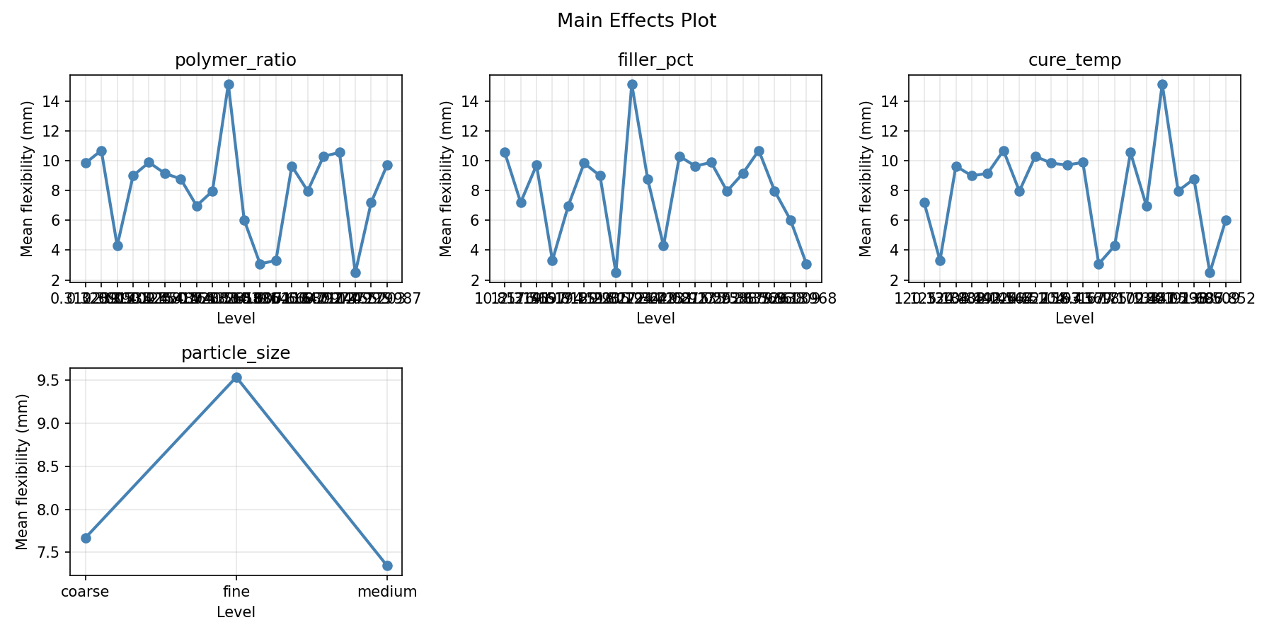
Response: flexibility

Flexibility is driven by a different balance of formulation factors, requiring trade-off analysis with tensile strength.

Pareto Chart

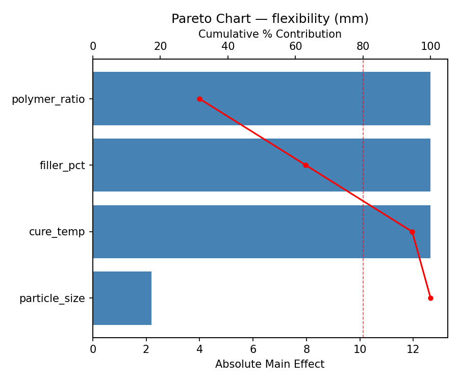
Main Effects Plot

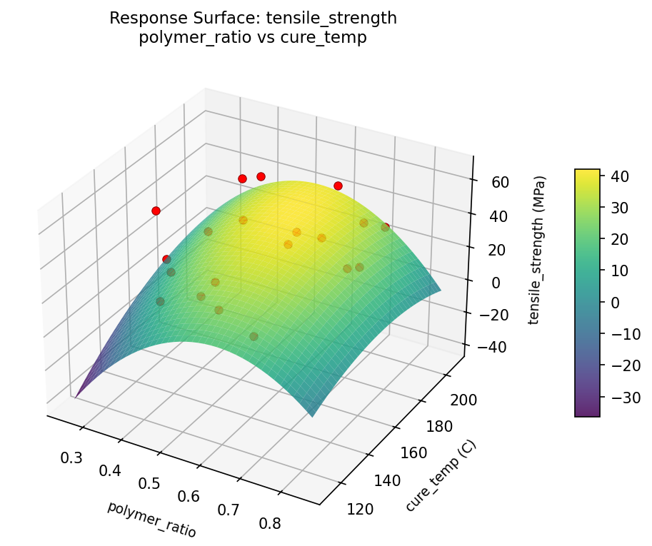
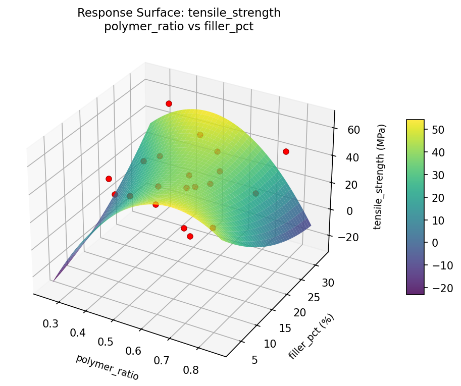
Response Surface Plots

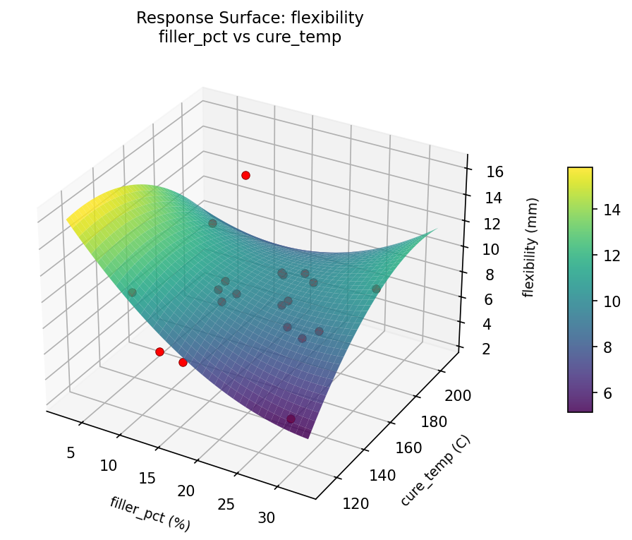
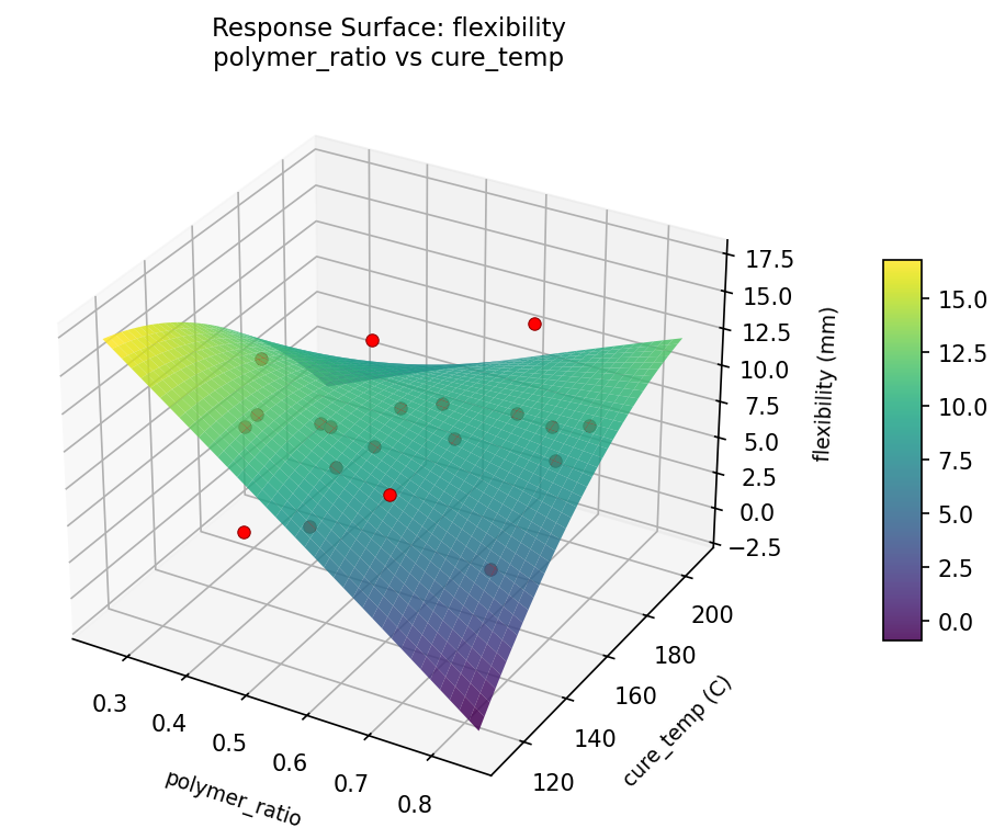
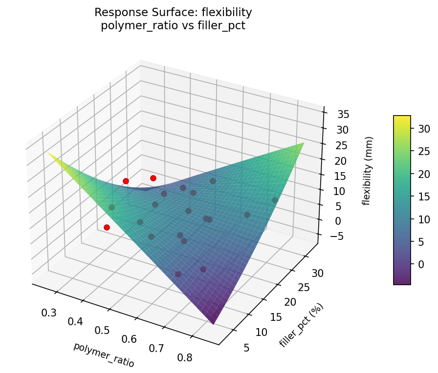
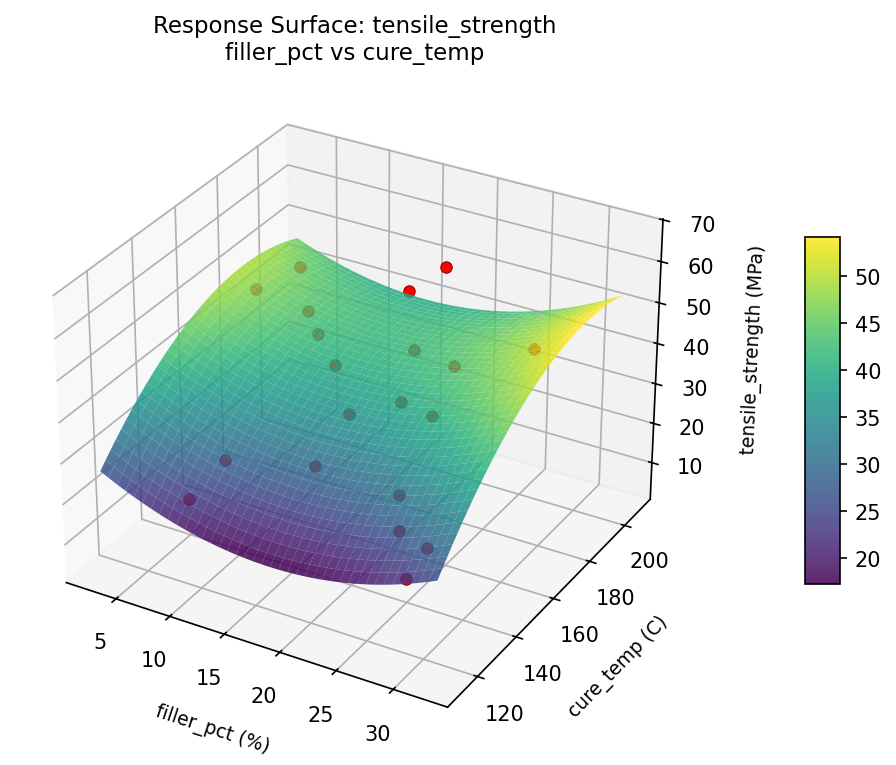
3D surfaces fitted with quadratic RSM. Red dots are observed data points.

📊

How to Read These Surfaces

Each plot shows predicted response (vertical axis) across two factors while other factors are held at center. Red dots are actual experimental observations.

Flat surface — these two factors have little effect on the response.
Tilted plane — strong linear effect; moving along one axis consistently changes the response.
Curved/domed surface — quadratic curvature; there is an optimum somewhere in the middle.
Saddle shape — significant interaction; the best setting of one factor depends on the other.
Red dots far from surface — poor model fit in that region; be cautious about predictions there.

tensile_strength (MPa) — R² = 0.905, Adj R² = 0.639
The model fits well — the surface shape is reliable.
Curvature detected in cure_temp, filler_pct — look for a peak or valley in the surface.
Strongest linear driver: filler_pct (increases tensile_strength).
Notable interaction: filler_pct × particle_size — the effect of one depends on the level of the other. Look for a twisted surface.

flexibility (mm) — R² = 0.626, Adj R² = -0.419
Moderate fit — surface shows general trends but some noise remains.
Curvature detected in polymer_ratio, cure_temp — look for a peak or valley in the surface.
Strongest linear driver: polymer_ratio (decreases flexibility).
Notable interaction: filler_pct × cure_temp — the effect of one depends on the level of the other. Look for a twisted surface.

flexibility: filler pct vs cure temp

flexibility: polymer ratio vs cure temp

flexibility: polymer ratio vs filler pct

tensile: strength filler pct vs cure temp

tensile: strength polymer ratio vs cure temp

tensile: strength polymer ratio vs filler pct

Full Analysis Output

doe analyze
=== Main Effects: tensile_strength ===
Factor                   Effect    Std Error   % Contribution
--------------------------------------------------------------
polymer_ratio           60.8000       3.9357            29.9%
filler_pct              60.8000       3.9357            29.9%
cure_temp               60.8000       3.9357            29.9%
particle_size           20.7429       3.9357            10.2%

=== Summary Statistics: tensile_strength ===

polymer_ratio:
  Level               N       Mean        Std        Min        Max
  ------------------------------------------------------------
30645             1    60.2000     0.0000    60.2000    60.2000
345057            1    57.9000     0.0000    57.9000    57.9000
364969            1    49.4000     0.0000    49.4000    49.4000
398627            1    30.2000     0.0000    30.2000    30.2000
412433            1    51.1000     0.0000    51.1000    51.1000
435932            1    20.7000     0.0000    20.7000    20.7000
457029            1     6.5000     0.0000     6.5000     6.5000
477081            1     5.0000     0.0000     5.0000     5.0000
500259            1    30.9000     0.0000    30.9000    30.9000
549414            1    21.2000     0.0000    21.2000    21.2000
565524            1    19.9000     0.0000    19.9000    19.9000
59909             1    65.8000     0.0000    65.8000    65.8000
608945            1    34.1000     0.0000    34.1000    34.1000
627461            1    24.6000     0.0000    24.6000    24.6000
661973            1    47.8000     0.0000    47.8000    47.8000
696713            1    47.1000     0.0000    47.1000    47.1000
716097            1    21.6000     0.0000    21.6000    21.6000
741222            1    50.2000     0.0000    50.2000    50.2000
758732            1    45.2000     0.0000    45.2000    45.2000
793704            1    30.3000     0.0000    30.3000    30.3000

filler_pct:
  Level               N       Mean        Std        Min        Max
  ------------------------------------------------------------
0774             1    47.1000     0.0000    47.1000    47.1000
7086             1    30.3000     0.0000    30.3000    30.3000
6117             1    21.2000     0.0000    21.2000    21.2000
4259             1    60.2000     0.0000    60.2000    60.2000
1864             1    21.6000     0.0000    21.6000    21.6000
1696             1    20.7000     0.0000    20.7000    20.7000
9415             1    24.6000     0.0000    24.6000    24.6000
0991             1    50.2000     0.0000    50.2000    50.2000
7811             1    65.8000     0.0000    65.8000    65.8000
4972             1    34.1000     0.0000    34.1000    34.1000
7419             1    47.8000     0.0000    47.8000    47.8000
9832             1    45.2000     0.0000    45.2000    45.2000
2071             1    30.9000     0.0000    30.9000    30.9000
4195             1    57.9000     0.0000    57.9000    57.9000
1025             1     6.5000     0.0000     6.5000     6.5000
6222             1    51.1000     0.0000    51.1000    51.1000
48476             1    30.2000     0.0000    30.2000    30.2000
96658             1     5.0000     0.0000     5.0000     5.0000
55985             1    19.9000     0.0000    19.9000    19.9000
99025             1    49.4000     0.0000    49.4000    49.4000

cure_temp:
  Level               N       Mean        Std        Min        Max
  ------------------------------------------------------------
363             1    20.7000     0.0000    20.7000    20.7000
967             1    47.1000     0.0000    47.1000    47.1000
352             1    30.9000     0.0000    30.9000    30.9000
74              1     6.5000     0.0000     6.5000     6.5000
442             1    47.8000     0.0000    47.8000    47.8000
466             1    49.4000     0.0000    49.4000    49.4000
706             1    24.6000     0.0000    24.6000    24.6000
101             1     5.0000     0.0000     5.0000     5.0000
254             1    34.1000     0.0000    34.1000    34.1000
829             1    21.2000     0.0000    21.2000    21.2000
748             1    30.2000     0.0000    30.2000    30.2000
685             1    60.2000     0.0000    60.2000    60.2000
313             1    65.8000     0.0000    65.8000    65.8000
847             1    45.2000     0.0000    45.2000    45.2000
763             1    57.9000     0.0000    57.9000    57.9000
397             1    51.1000     0.0000    51.1000    51.1000
257             1    21.6000     0.0000    21.6000    21.6000
124             1    19.9000     0.0000    19.9000    19.9000
231             1    50.2000     0.0000    50.2000    50.2000
953             1    30.3000     0.0000    30.3000    30.3000

particle_size:
  Level               N       Mean        Std        Min        Max
  ------------------------------------------------------------
  coarse              7    43.4429     7.9227    30.3000    50.2000
  fine                6    42.7833    20.7670    20.7000    65.8000
  medium              7    22.7000    15.5521     5.0000    51.1000

=== Main Effects: flexibility ===
Factor                   Effect    Std Error   % Contribution
--------------------------------------------------------------
polymer_ratio           12.6500       0.6906            32.4%
filler_pct              12.6500       0.6906            32.4%
cure_temp               12.6500       0.6906            32.4%
particle_size            1.0757       0.6906             2.8%

=== Summary Statistics: flexibility ===

polymer_ratio:
  Level               N       Mean        Std        Min        Max
  ------------------------------------------------------------
30645             1     2.4900     0.0000     2.4900     2.4900
345057            1     6.9800     0.0000     6.9800     6.9800
364969            1     9.6400     0.0000     9.6400     9.6400
398627            1     6.0200     0.0000     6.0200     6.0200
412433            1     7.2000     0.0000     7.2000     7.2000
435932            1    15.1400     0.0000    15.1400    15.1400
457029            1     9.1500     0.0000     9.1500     9.1500
477081            1    10.5500     0.0000    10.5500    10.5500
500259            1     8.9900     0.0000     8.9900     8.9900
549414            1    10.6900     0.0000    10.6900    10.6900
565524            1     7.9600     0.0000     7.9600     7.9600
59909             1     3.0800     0.0000     3.0800     3.0800
608945            1     3.3100     0.0000     3.3100     3.3100
627461            1    10.3000     0.0000    10.3000    10.3000
661973            1     8.7800     0.0000     8.7800     8.7800
696713            1     4.2900     0.0000     4.2900     4.2900
716097            1     9.8900     0.0000     9.8900     9.8900
741222            1     9.8400     0.0000     9.8400     9.8400
758732            1     7.9700     0.0000     7.9700     7.9700
793704            1     9.7100     0.0000     9.7100     9.7100

filler_pct:
  Level               N       Mean        Std        Min        Max
  ------------------------------------------------------------
0774             1     4.2900     0.0000     4.2900     4.2900
7086             1     9.7100     0.0000     9.7100     9.7100
6117             1    10.6900     0.0000    10.6900    10.6900
4259             1     2.4900     0.0000     2.4900     2.4900
1864             1     9.8900     0.0000     9.8900     9.8900
1696             1    15.1400     0.0000    15.1400    15.1400
9415             1    10.3000     0.0000    10.3000    10.3000
0991             1     9.8400     0.0000     9.8400     9.8400
7811             1     3.0800     0.0000     3.0800     3.0800
4972             1     3.3100     0.0000     3.3100     3.3100
7419             1     8.7800     0.0000     8.7800     8.7800
9832             1     7.9700     0.0000     7.9700     7.9700
2071             1     8.9900     0.0000     8.9900     8.9900
4195             1     6.9800     0.0000     6.9800     6.9800
1025             1     9.1500     0.0000     9.1500     9.1500
6222             1     7.2000     0.0000     7.2000     7.2000
48476             1     6.0200     0.0000     6.0200     6.0200
96658             1    10.5500     0.0000    10.5500    10.5500
55985             1     7.9600     0.0000     7.9600     7.9600
99025             1     9.6400     0.0000     9.6400     9.6400

cure_temp:
  Level               N       Mean        Std        Min        Max
  ------------------------------------------------------------
363             1    15.1400     0.0000    15.1400    15.1400
967             1     4.2900     0.0000     4.2900     4.2900
352             1     8.9900     0.0000     8.9900     8.9900
74              1     9.1500     0.0000     9.1500     9.1500
442             1     8.7800     0.0000     8.7800     8.7800
466             1     9.6400     0.0000     9.6400     9.6400
706             1    10.3000     0.0000    10.3000    10.3000
101             1    10.5500     0.0000    10.5500    10.5500
254             1     3.3100     0.0000     3.3100     3.3100
829             1    10.6900     0.0000    10.6900    10.6900
748             1     6.0200     0.0000     6.0200     6.0200
685             1     2.4900     0.0000     2.4900     2.4900
313             1     3.0800     0.0000     3.0800     3.0800
847             1     7.9700     0.0000     7.9700     7.9700
763             1     6.9800     0.0000     6.9800     6.9800
397             1     7.2000     0.0000     7.2000     7.2000
257             1     9.8900     0.0000     9.8900     9.8900
124             1     7.9600     0.0000     7.9600     7.9600
231             1     9.8400     0.0000     9.8400     9.8400
953             1     9.7100     0.0000     9.7100     9.7100

particle_size:
  Level               N       Mean        Std        Min        Max
  ------------------------------------------------------------
  coarse              7     7.6486     2.7235     3.3100     9.8400
  fine                6     7.8950     4.7903     2.4900    15.1400
  medium              7     8.7243     1.7116     6.0200    10.5500

Optimization Recommendations

doe optimize
=== Optimization: tensile_strength ===
Direction: maximize

Best observed run: #12
  polymer_ratio = 0.734037
  filler_pct = 12.1712
  cure_temp = 135.352
  particle_size = coarse
  Value: 65.8

RSM Model (linear, R² = 0.14):
  Coefficients:
    intercept:  +36.0046
    polymer_ratio:  +5.2791
    filler_pct:  -8.0744
    cure_temp:  -1.3667
    particle_size:  +1.6144
  Predicted optimum:
    polymer_ratio = 0.799682
    filler_pct = 6.98001
    cure_temp = 193.433
    particle_size = medium
    Predicted value: 48.5444

Factor importance:
  1. polymer_ratio  (effect: 60.8, contribution: 32.4%)
  2. filler_pct  (effect: 60.8, contribution: 32.4%)
  3. cure_temp  (effect: 60.8, contribution: 32.4%)
  4. particle_size  (effect: 5.5, contribution: 2.9%)

=== Optimization: flexibility ===
Direction: maximize

Best observed run: #7
  polymer_ratio = 0.595795
  filler_pct = 17.5526
  cure_temp = 198.806
  particle_size = medium
  Value: 15.14

RSM Model (linear, R² = 0.24):
  Coefficients:
    intercept:  +8.0600
    polymer_ratio:  -0.7442
    filler_pct:  +0.9248
    cure_temp:  +1.9985
    particle_size:  -0.6976
  Predicted optimum:
    polymer_ratio = 0.483128
    filler_pct = 21.5583
    cure_temp = 186.217
    particle_size = coarse
    Predicted value: 10.5668

Factor importance:
  1. polymer_ratio  (effect: 12.7, contribution: 32.1%)
  2. filler_pct  (effect: 12.7, contribution: 32.1%)
  3. cure_temp  (effect: 12.7, contribution: 32.1%)
  4. particle_size  (effect: 1.5, contribution: 3.8%)

Multi-Objective Optimization

When responses compete, Derringer–Suich desirability finds the best compromise. Each response is scaled to a 0–1 desirability, then combined via a weighted geometric mean.

Overall Desirability

D = 0.6433

Per-Response Desirability

Response	Weight	Desirability	Predicted	Dir
`tensile_strength`	1.5	0.7213	50.20 0.7213 50.20 MPa	↑
`flexibility`	1.5	0.5737	9.84 0.5737 9.84 mm	↑

Recommended Settings

Factor	Value
`polymer_ratio`	0.450642
`filler_pct`	21.1846 %
`cure_temp`	168.139 C
`particle_size`	fine

Source: from observed run #2

Trade-off Summary

Sacrifice = how much worse than single-objective best.

Response	Predicted	Best Observed	Sacrifice
`flexibility`	9.84	15.14	+5.30

Top 3 Runs by Desirability

Run	D	Factor Settings
#3	0.6299	polymer_ratio=0.727739, filler_pct=27.6875, cure_temp=164.744, particle_size=medium
#17	0.5839	polymer_ratio=0.378219, filler_pct=29.8691, cure_temp=127.804, particle_size=medium

Model Quality

Response	R²	Type
`flexibility`	0.3726	linear

Full Multi-Objective Output

doe optimize --multi
============================================================
MULTI-OBJECTIVE OPTIMIZATION
Method: Derringer-Suich Desirability Function
============================================================

Overall desirability: D = 0.6433

Response                  Weight Desirability    Predicted  Direction
---------------------------------------------------------------------
tensile_strength             1.5       0.7213       50.20 MPa   ↑
flexibility                  1.5       0.5737        9.84 mm   ↑

Recommended settings:
  polymer_ratio = 0.450642
  filler_pct = 21.1846 %
  cure_temp = 168.139 C
  particle_size = fine
  (from observed run #2)

Trade-off summary:
  tensile_strength: 50.20 (best observed: 65.80, sacrifice: +15.60)
  flexibility: 9.84 (best observed: 15.14, sacrifice: +5.30)

Model quality:
  tensile_strength: R² = 0.2491 (linear)
  flexibility: R² = 0.3726 (linear)

Top 3 observed runs by overall desirability:
  1. Run #2 (D=0.6433): polymer_ratio=0.450642, filler_pct=21.1846, cure_temp=168.139, particle_size=fine
  2. Run #3 (D=0.6299): polymer_ratio=0.727739, filler_pct=27.6875, cure_temp=164.744, particle_size=medium
  3. Run #17 (D=0.5839): polymer_ratio=0.378219, filler_pct=29.8691, cure_temp=127.804, particle_size=medium