Summary
This experiment investigates drip irrigation scheduling. Central composite design to minimize water usage and maximize crop yield by tuning drip rate, interval, and emitter spacing.
The design varies 3 factors: drip rate (L/hr), ranging from 1 to 4, interval hrs (hrs), ranging from 6 to 48, and emitter spacing (cm), ranging from 20 to 50. The goal is to optimize 2 responses: water use L (L/m2/wk) (minimize) and crop yield (kg/m2) (maximize). Fixed conditions held constant across all runs include crop = strawberry, season = summer.
A Central Composite Design (CCD) was selected to fit a full quadratic response surface model, including curvature and interaction effects. With 3 factors this produces 22 runs including center points and axial (star) points that extend beyond the factorial range.
Quadratic response surface models were fitted to capture potential curvature and factor interactions. The RSM contour plots below visualize how pairs of factors jointly affect each response.
Key Findings
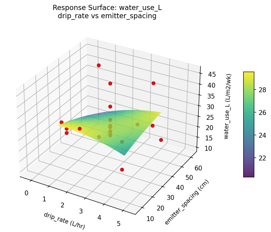
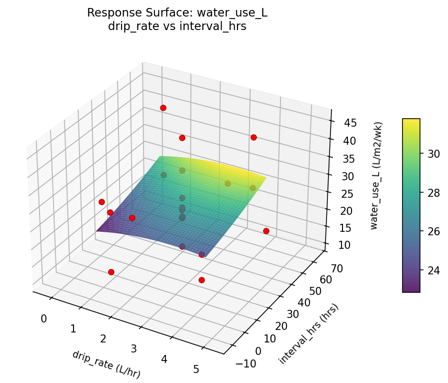
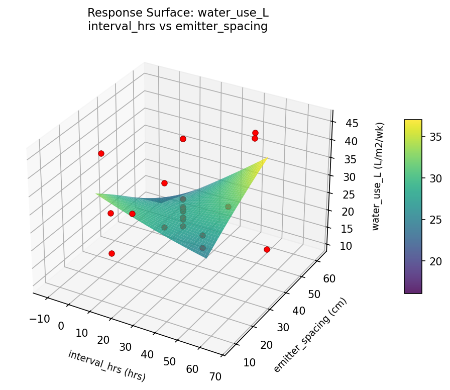
For water use L, the most influential factors were emitter spacing (46.4%), drip rate (41.9%), interval hrs (11.8%). The best observed value was 10.5 (at drip rate = 2.5, interval hrs = 27, emitter spacing = 62.3861).
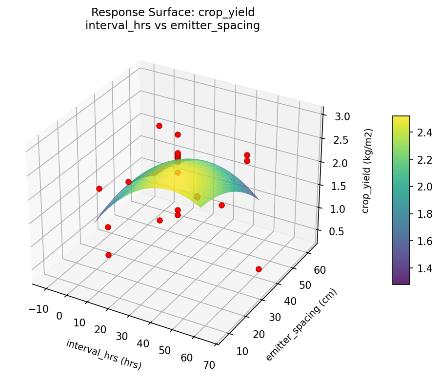
For crop yield, the most influential factors were emitter spacing (43.1%), drip rate (32.6%), interval hrs (24.4%). The best observed value was 2.97 (at drip rate = 2.5, interval hrs = -11.3406, emitter spacing = 35).
Recommended Next Steps
- Run confirmation experiments at the predicted optimal settings to validate the model.
- Consider whether any fixed factors should be varied in a future study.
Experimental Setup
Factors
| Factor | Low | High | Unit |
|---|
drip_rate | 1 | 4 | L/hr |
interval_hrs | 6 | 48 | hrs |
emitter_spacing | 20 | 50 | cm |
Fixed: crop = strawberry, season = summer
Responses
| Response | Direction | Unit |
|---|
water_use_L | ↓ minimize | L/m2/wk |
crop_yield | ↑ maximize | kg/m2 |
Configuration
{
"metadata": {
"name": "Drip Irrigation Scheduling",
"description": "Central composite design to minimize water usage and maximize crop yield by tuning drip rate, interval, and emitter spacing"
},
"factors": [
{
"name": "drip_rate",
"levels": [
"1",
"4"
],
"type": "continuous",
"unit": "L/hr"
},
{
"name": "interval_hrs",
"levels": [
"6",
"48"
],
"type": "continuous",
"unit": "hrs"
},
{
"name": "emitter_spacing",
"levels": [
"20",
"50"
],
"type": "continuous",
"unit": "cm"
}
],
"fixed_factors": {
"crop": "strawberry",
"season": "summer"
},
"responses": [
{
"name": "water_use_L",
"optimize": "minimize",
"unit": "L/m2/wk"
},
{
"name": "crop_yield",
"optimize": "maximize",
"unit": "kg/m2"
}
],
"settings": {
"operation": "central_composite",
"test_script": "use_cases/104_irrigation_scheduling/sim.sh"
}
}
Experimental Matrix
The Central Composite Design produces 22 runs. Each row is one experiment with specific factor settings.
| Run | drip_rate | interval_hrs | emitter_spacing |
|---|
| 1 | 2.5 | 27 | 35 |
| 2 | 4 | 6 | 50 |
| 3 | 1 | 48 | 20 |
| 4 | 2.5 | 65.3406 | 35 |
| 5 | 2.5 | 27 | 35 |
| 6 | -0.238613 | 27 | 35 |
| 7 | 2.5 | 27 | 7.61387 |
| 8 | 2.5 | 27 | 35 |
| 9 | 4 | 48 | 20 |
| 10 | 5.23861 | 27 | 35 |
| 11 | 2.5 | 27 | 35 |
| 12 | 2.5 | -11.3406 | 35 |
| 13 | 2.5 | 27 | 35 |
| 14 | 1 | 6 | 50 |
| 15 | 2.5 | 27 | 35 |
| 16 | 4 | 6 | 20 |
| 17 | 2.5 | 27 | 62.3861 |
| 18 | 4 | 48 | 50 |
| 19 | 2.5 | 27 | 35 |
| 20 | 1 | 6 | 20 |
| 21 | 1 | 48 | 50 |
| 22 | 2.5 | 27 | 35 |
Step-by-Step Workflow
1
Preview the design
$ doe info --config use_cases/104_irrigation_scheduling/config.json
2
Generate the runner script
$ doe generate --config use_cases/104_irrigation_scheduling/config.json \
--output use_cases/104_irrigation_scheduling/results/run.sh --seed 42
3
Execute the experiments
$ bash use_cases/104_irrigation_scheduling/results/run.sh
4
Analyze results
$ doe analyze --config use_cases/104_irrigation_scheduling/config.json
5
Get optimization recommendations
$ doe optimize --config use_cases/104_irrigation_scheduling/config.json
6
Multi-objective optimization
With 2 competing responses, use --multi to find the best compromise via Derringer–Suich desirability.
$ doe optimize --config use_cases/104_irrigation_scheduling/config.json --multi
7
Generate the HTML report
$ doe report --config use_cases/104_irrigation_scheduling/config.json \
--output use_cases/104_irrigation_scheduling/results/report.html
Features Exercised
| Feature | Value |
|---|
| Design type | central_composite |
| Factor types | continuous (all 3) |
| Arg style | double-dash |
| Responses | 2 (water_use_L ↓, crop_yield ↑) |
| Total runs | 22 |
Analysis Results
Generated from actual experiment runs using the DOE Helper Tool.
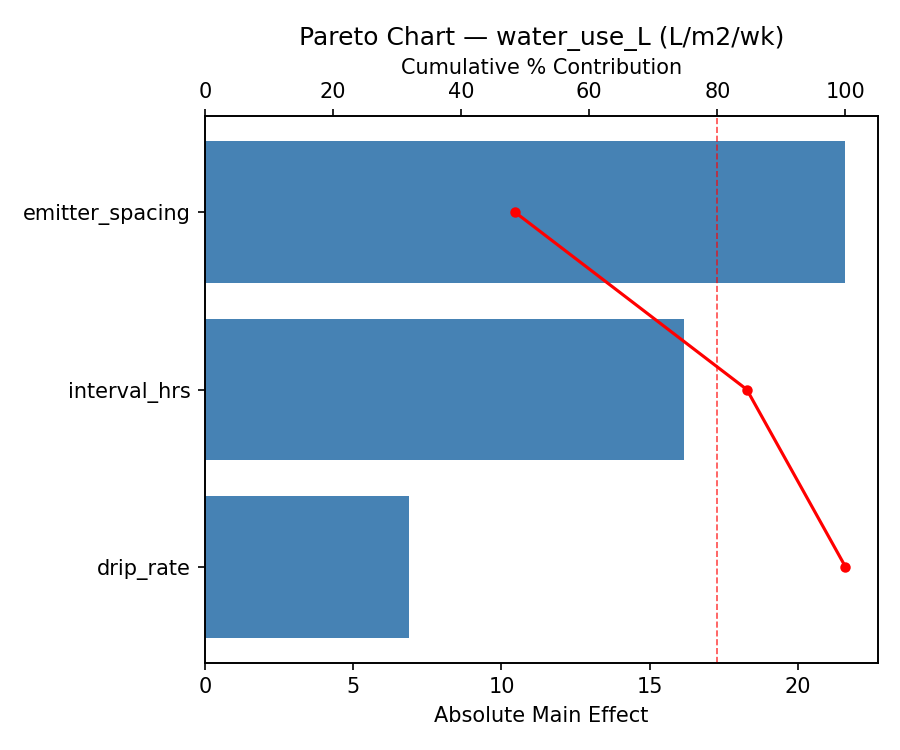
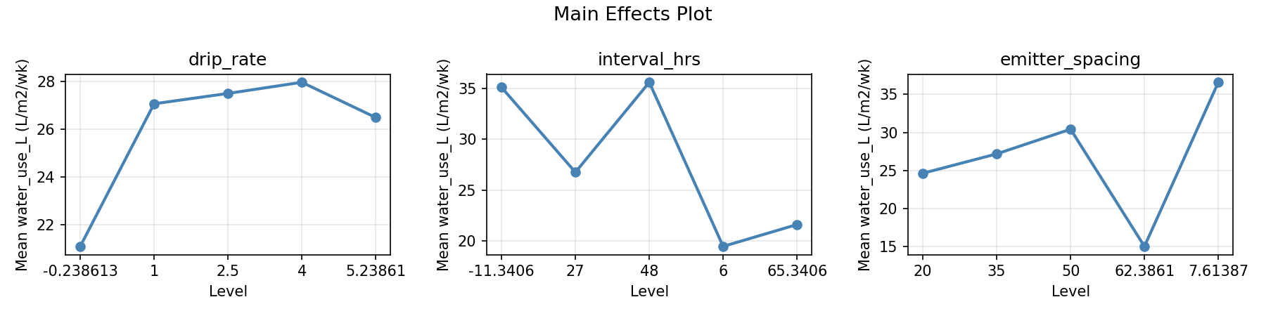
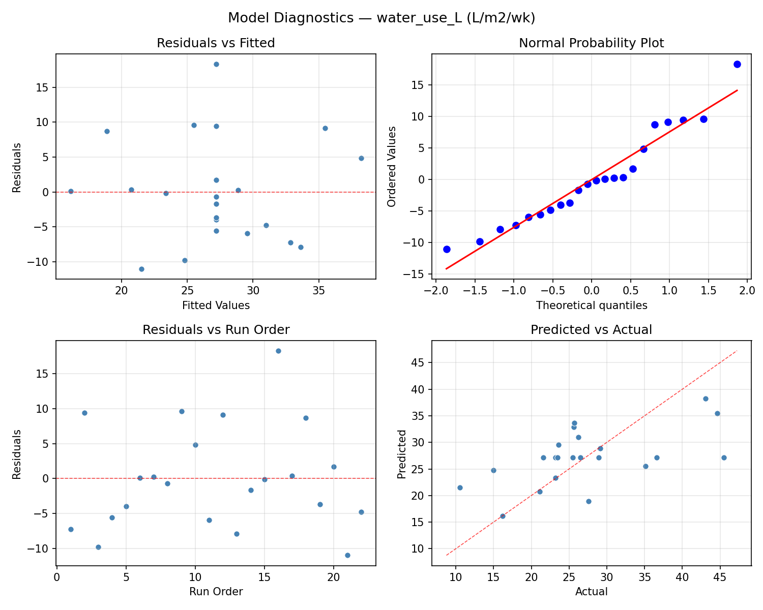
Response: water_use_L
Top factors: emitter_spacing (46.4%), drip_rate (41.9%), interval_hrs (11.8%).
ANOVA
| Source | DF | SS | MS | F | p-value |
|---|
| Source | DF | SS | MS | F | p-value |
| drip_rate | 4 | 365.5720 | 91.3930 | 1.353 | 0.3233 |
| interval_hrs | 4 | 51.9020 | 12.9755 | 0.192 | 0.9365 |
| emitter_spacing | 4 | 543.3945 | 135.8486 | 2.011 | 0.1765 |
| Lack | of | Fit | 2 | 299.2352 | 149.6176 |
| Pure | Error | 7 | 472.9150 | | |
| Error | 9 | 772.1502 | 67.5593 | | |
| Total | 21 | 1733.0186 | 82.5247 | | |
Pareto Chart
Main Effects Plot
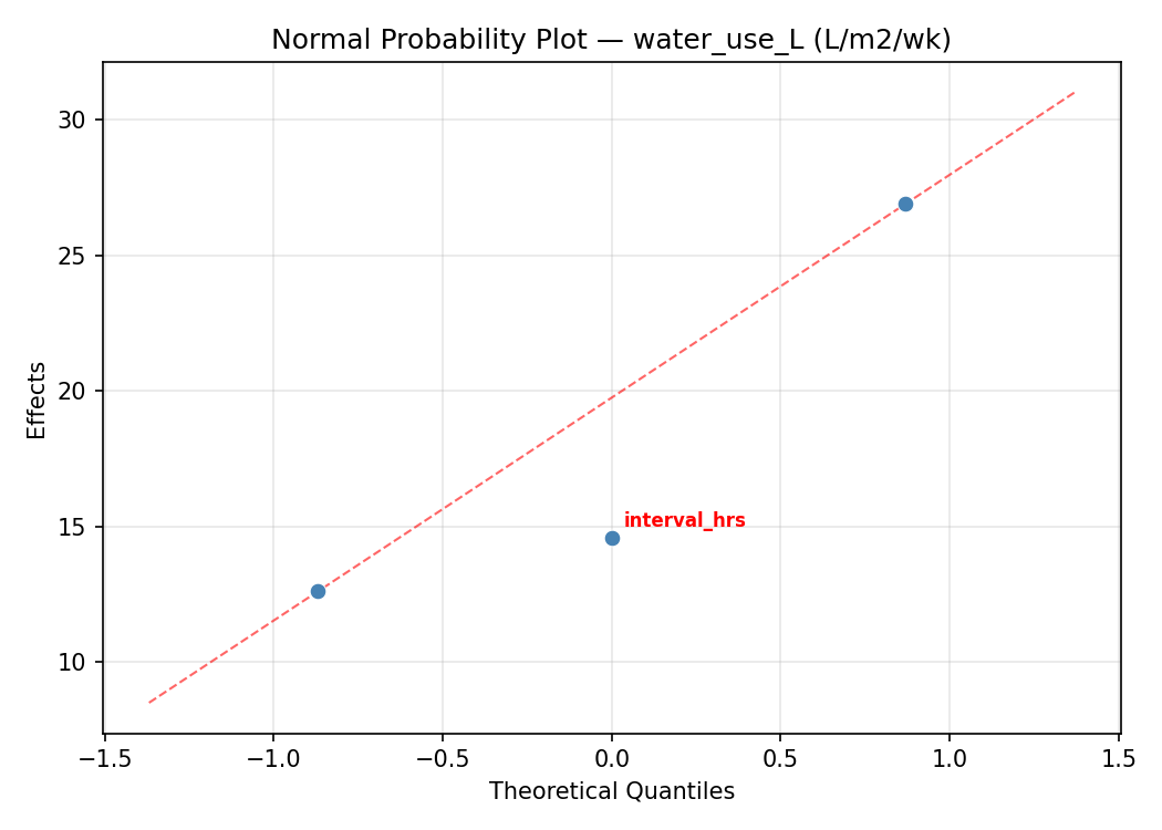
Normal Probability Plot of Effects
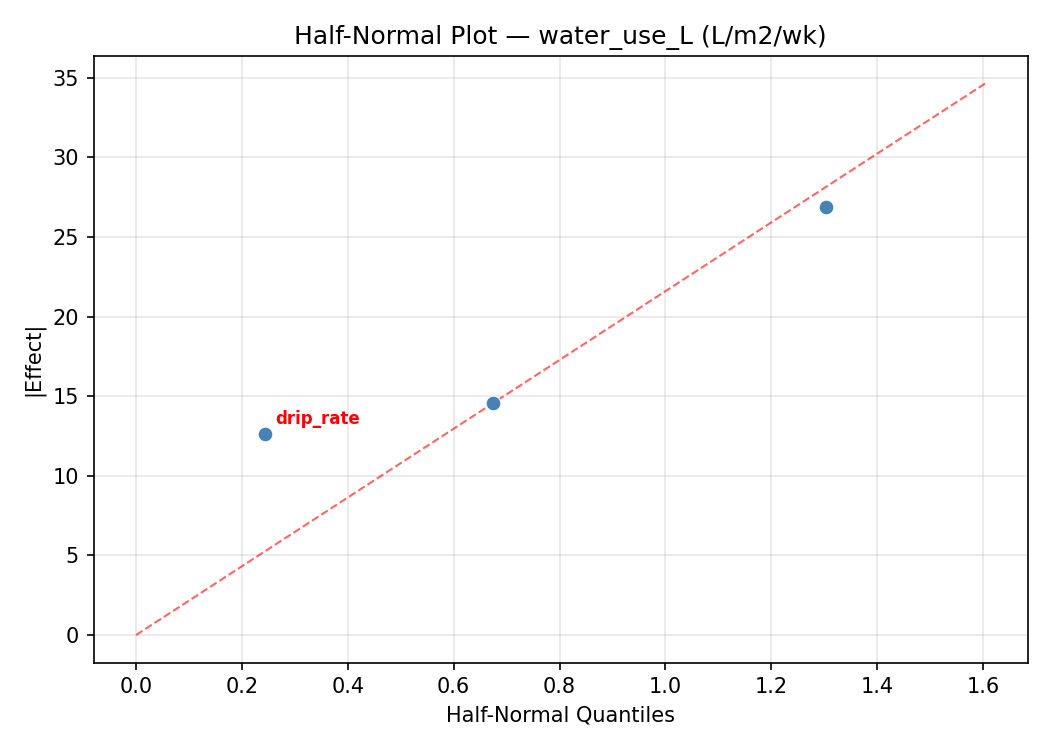
Half-Normal Plot of Effects
Model Diagnostics
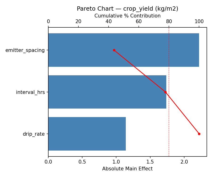
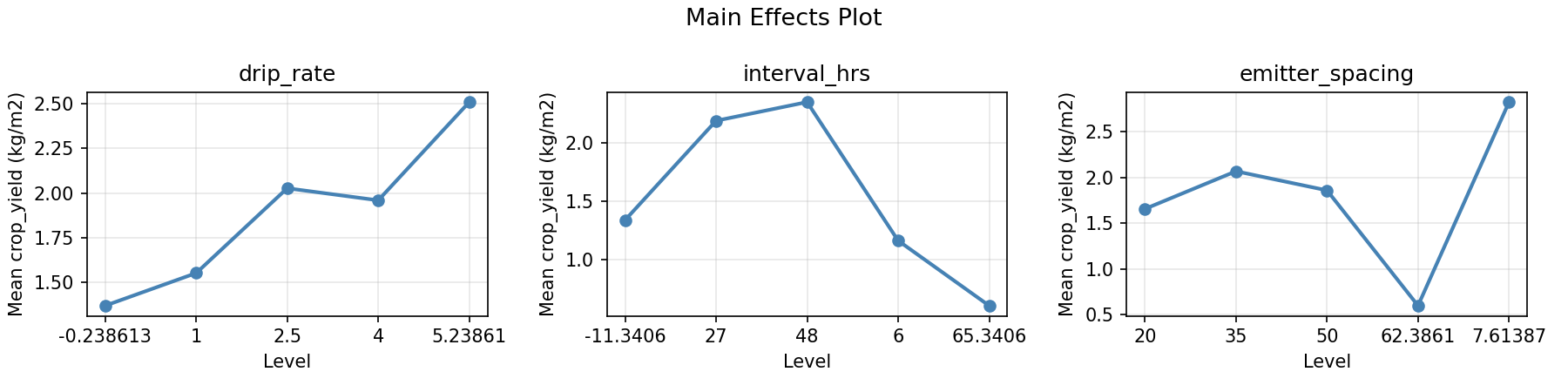
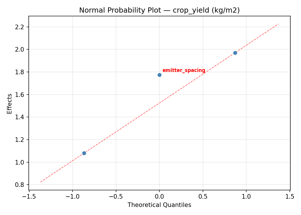
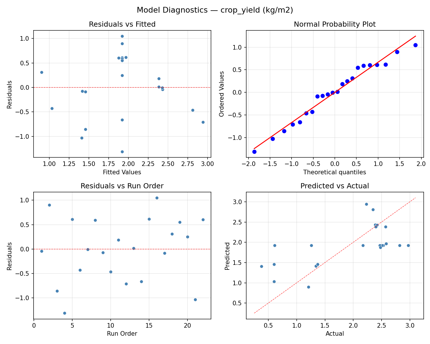
Response: crop_yield
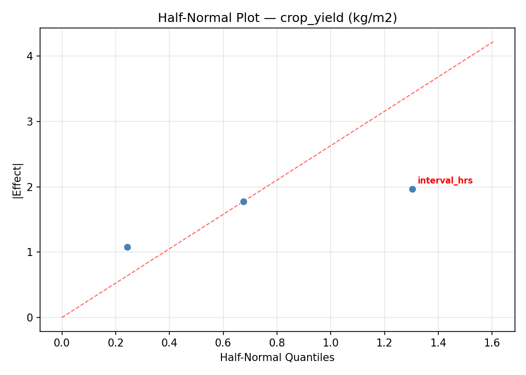
Top factors: emitter_spacing (43.1%), drip_rate (32.6%), interval_hrs (24.4%).
ANOVA
| Source | DF | SS | MS | F | p-value |
|---|
| Source | DF | SS | MS | F | p-value |
| drip_rate | 4 | 2.2759 | 0.5690 | 0.671 | 0.6283 |
| interval_hrs | 4 | 3.2677 | 0.8169 | 0.964 | 0.4724 |
| emitter_spacing | 4 | 3.4045 | 0.8511 | 1.004 | 0.4540 |
| Lack | of | Fit | 2 | 0.0000 | 0.0000 |
| Pure | Error | 7 | 5.9346 | | |
| Error | 9 | 5.3546 | 0.8478 | | |
| Total | 21 | 14.3028 | 0.6811 | | |
Pareto Chart
Main Effects Plot
Normal Probability Plot of Effects
Half-Normal Plot of Effects
Model Diagnostics
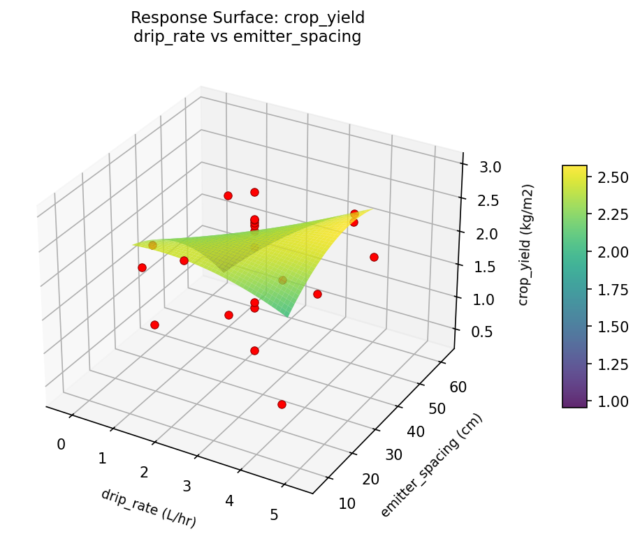
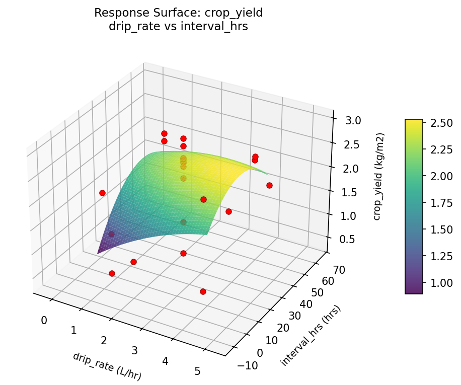
Response Surface Plots
3D surfaces fitted with quadratic RSM. Red dots are observed data points.
crop yield drip rate vs emitter spacing
crop yield drip rate vs interval hrs
crop yield interval hrs vs emitter spacing
water use L drip rate vs emitter spacing
water use L drip rate vs interval hrs
water use L interval hrs vs emitter spacing
Multi-Objective Optimization
When responses compete, Derringer–Suich desirability finds the best compromise.
Each response is scaled to a 0–1 desirability, then combined via a weighted geometric mean.
Overall Desirability
D = 0.8073
Per-Response Desirability
| Response | Weight | Desirability | Predicted | Dir |
|---|
water_use_L |
1.0 |
|
22.32 0.6475 22.32 L/m2/wk |
↓ |
crop_yield |
1.5 |
|
2.91 0.9351 2.91 kg/m2 |
↑ |
Recommended Settings
| Factor | Value |
|---|
drip_rate | 1 L/hr |
interval_hrs | 48 hrs |
emitter_spacing | 32 cm |
Source: from RSM model prediction
Trade-off Summary
Sacrifice = how much worse than single-objective best.
| Response | Predicted | Best Observed | Sacrifice |
|---|
crop_yield | 2.91 | 2.97 | +0.06 |
Top 3 Runs by Desirability
| Run | D | Factor Settings |
|---|
| #11 | 0.7274 | drip_rate=1, interval_hrs=48, emitter_spacing=50 |
| #5 | 0.7247 | drip_rate=2.5, interval_hrs=27, emitter_spacing=35 |
Model Quality
| Response | R² | Type |
|---|
crop_yield | 0.3956 | quadratic |
Full Multi-Objective Output
============================================================
MULTI-OBJECTIVE OPTIMIZATION
Method: Derringer-Suich Desirability Function
============================================================
Overall desirability: D = 0.8073
Response Weight Desirability Predicted Direction
---------------------------------------------------------------------
water_use_L 1.0 0.6475 22.32 L/m2/wk ↓
crop_yield 1.5 0.9351 2.91 kg/m2 ↑
Recommended settings:
drip_rate = 1 L/hr
interval_hrs = 48 hrs
emitter_spacing = 32 cm
(from RSM model prediction)
Trade-off summary:
water_use_L: 22.32 (best observed: 10.50, sacrifice: +11.82)
crop_yield: 2.91 (best observed: 2.97, sacrifice: +0.06)
Model quality:
water_use_L: R² = 0.1624 (linear)
crop_yield: R² = 0.3956 (quadratic)
Top 3 observed runs by overall desirability:
1. Run #15 (D=0.7342): drip_rate=2.5, interval_hrs=27, emitter_spacing=35
2. Run #11 (D=0.7274): drip_rate=1, interval_hrs=48, emitter_spacing=50
3. Run #5 (D=0.7247): drip_rate=2.5, interval_hrs=27, emitter_spacing=35
Full Analysis Output
=== Main Effects: water_use_L ===
Factor Effect Std Error % Contribution
--------------------------------------------------------------
emitter_spacing 23.2250 1.9368 46.4%
drip_rate 20.9750 1.9368 41.9%
interval_hrs 5.9000 1.9368 11.8%
=== ANOVA Table: water_use_L ===
Source DF SS MS F p-value
-----------------------------------------------------------------------------
drip_rate 4 365.5720 91.3930 1.353 0.3233
interval_hrs 4 51.9020 12.9755 0.192 0.9365
emitter_spacing 4 543.3945 135.8486 2.011 0.1765
Lack of Fit 2 299.2352 149.6176 2.215 0.1798
Pure Error 7 472.9150 67.5593
Error 9 772.1502 67.5593
Total 21 1733.0186 82.5247
=== Summary Statistics: water_use_L ===
drip_rate:
Level N Mean Std Min Max
------------------------------------------------------------
-0.238613 1 25.5000 0.0000 25.5000 25.5000
1 4 28.3500 9.8348 23.2000 43.1000
2.5 12 26.6583 9.5506 10.5000 45.5000
4 4 23.6250 4.9641 16.2000 26.5000
5.23861 1 44.6000 0.0000 44.6000 44.6000
interval_hrs:
Level N Mean Std Min Max
------------------------------------------------------------
-11.3406 1 29.1000 0.0000 29.1000 29.1000
27 12 28.1417 10.7968 10.5000 45.5000
48 4 24.8750 1.7154 23.2000 26.5000
6 4 27.1000 11.4020 16.2000 43.1000
65.3406 1 23.2000 0.0000 23.2000 23.2000
emitter_spacing:
Level N Mean Std Min Max
------------------------------------------------------------
20 4 22.2750 4.2688 16.2000 26.2000
35 12 25.7833 9.0007 10.5000 44.6000
50 4 29.7000 9.0152 23.6000 43.1000
62.3861 1 45.5000 0.0000 45.5000 45.5000
7.61387 1 35.1000 0.0000 35.1000 35.1000
=== Main Effects: crop_yield ===
Factor Effect Std Error % Contribution
--------------------------------------------------------------
emitter_spacing 1.6300 0.1759 43.1%
drip_rate 1.2325 0.1759 32.6%
interval_hrs 0.9217 0.1759 24.4%
=== ANOVA Table: crop_yield ===
Source DF SS MS F p-value
-----------------------------------------------------------------------------
drip_rate 4 2.2759 0.5690 0.671 0.6283
interval_hrs 4 3.2677 0.8169 0.964 0.4724
emitter_spacing 4 3.4045 0.8511 1.004 0.4540
Lack of Fit 2 0.0000 0.0000 0.000 1.0000
Pure Error 7 5.9346 0.8478
Error 9 5.3546 0.8478
Total 21 14.3028 0.6811
=== Summary Statistics: crop_yield ===
drip_rate:
Level N Mean Std Min Max
------------------------------------------------------------
-0.238613 1 1.2600 0.0000 1.2600 1.2600
1 4 2.4925 0.1072 2.3500 2.5800
2.5 12 1.7350 0.9239 0.3800 2.9700
4 4 1.9950 0.9314 0.6000 2.5100
5.23861 1 2.2300 0.0000 2.2300 2.2300
interval_hrs:
Level N Mean Std Min Max
------------------------------------------------------------
-11.3406 1 2.4200 0.0000 2.4200 2.4200
27 12 1.6133 0.8833 0.3800 2.9700
48 4 2.5350 0.0480 2.4800 2.5800
6 4 1.9525 0.9030 0.6000 2.4700
65.3406 1 2.5300 0.0000 2.5300 2.5300
emitter_spacing:
Level N Mean Std Min Max
------------------------------------------------------------
20 4 2.0325 0.9563 0.6000 2.5800
35 12 1.6667 0.8593 0.3800 2.8200
50 4 2.4550 0.1025 2.3500 2.5700
62.3861 1 2.9700 0.0000 2.9700 2.9700
7.61387 1 1.3400 0.0000 1.3400 1.3400
Optimization Recommendations
=== Optimization: water_use_L ===
Direction: minimize
Best observed run: #21
drip_rate = 2.5
interval_hrs = 27
emitter_spacing = 62.3861
Value: 10.5
RSM Model (linear, R² = 0.3850, Adj R² = 0.2824):
Coefficients:
intercept +27.1773
drip_rate -0.4757
interval_hrs -2.4977
emitter_spacing -6.2468
RSM Model (quadratic, R² = 0.4962, Adj R² = 0.1184):
Coefficients:
intercept +28.2260
drip_rate -0.4757
interval_hrs -2.4977
emitter_spacing -6.2468
drip_rate*interval_hrs -0.9625
drip_rate*emitter_spacing +2.0625
interval_hrs*emitter_spacing -0.7875
drip_rate^2 -1.8193
interval_hrs^2 +1.4357
emitter_spacing^2 -1.1893
Curvature analysis:
drip_rate coef=-1.8193 concave (has a maximum)
interval_hrs coef=+1.4357 convex (has a minimum)
emitter_spacing coef=-1.1893 concave (has a maximum)
Notable interactions:
drip_rate*emitter_spacing coef=+2.0625 (synergistic)
drip_rate*interval_hrs coef=-0.9625 (antagonistic)
interval_hrs*emitter_spacing coef=-0.7875 (antagonistic)
Predicted optimum (from linear model, at observed points):
drip_rate = 2.5
interval_hrs = 27
emitter_spacing = 7.61387
Predicted value: 38.5823
Surface optimum (via L-BFGS-B, linear model):
drip_rate = 4
interval_hrs = 48
emitter_spacing = 50
Predicted value: 17.9571
Model quality: Weak fit — consider adding center points or using a different design.
Factor importance:
1. emitter_spacing (effect: 32.6, contribution: 54.6%)
2. interval_hrs (effect: 21.0, contribution: 35.1%)
3. drip_rate (effect: 6.1, contribution: 10.3%)
=== Optimization: crop_yield ===
Direction: maximize
Best observed run: #16
drip_rate = 2.5
interval_hrs = -11.3406
emitter_spacing = 35
Value: 2.97
RSM Model (linear, R² = 0.2813, Adj R² = 0.1615):
Coefficients:
intercept +1.9209
drip_rate +0.1631
interval_hrs -0.0702
emitter_spacing -0.4927
RSM Model (quadratic, R² = 0.6060, Adj R² = 0.3105):
Coefficients:
intercept +1.8868
drip_rate +0.1631
interval_hrs -0.0702
emitter_spacing -0.4927
drip_rate*interval_hrs +0.4888
drip_rate*emitter_spacing +0.0162
interval_hrs*emitter_spacing +0.2837
drip_rate^2 +0.1185
interval_hrs^2 +0.1635
emitter_spacing^2 -0.2310
Curvature analysis:
emitter_spacing coef=-0.2310 concave (has a maximum)
interval_hrs coef=+0.1635 convex (has a minimum)
drip_rate coef=+0.1185 convex (has a minimum)
Notable interactions:
drip_rate*interval_hrs coef=+0.4888 (synergistic)
Predicted optimum (from quadratic model, at observed points):
drip_rate = 1
interval_hrs = 6
emitter_spacing = 20
Predicted value: 3.1265
Surface optimum (via L-BFGS-B, quadratic model):
drip_rate = 1
interval_hrs = 6
emitter_spacing = 20
Predicted value: 3.1265
Model quality: Moderate fit — use predictions directionally, not precisely.
Factor importance:
1. emitter_spacing (effect: 2.0, contribution: 45.4%)
2. interval_hrs (effect: 1.2, contribution: 28.6%)
3. drip_rate (effect: 1.1, contribution: 25.9%)