Summary
This experiment investigates greenhouse climate control. Plackett-Burman screening of ventilation rate, shade cloth, CO2 enrichment, heating setpoint, and misting frequency for plant growth and energy cost.
The design varies 5 factors: vent rate (ach), ranging from 5 to 30, shade pct (%), ranging from 0 to 60, co2 ppm (ppm), ranging from 400 to 1200, heat setpoint (C), ranging from 15 to 25, and mist freq (per_day), ranging from 0 to 12. The goal is to optimize 2 responses: growth index (pts) (maximize) and energy cost (USD/day) (minimize). Fixed conditions held constant across all runs include greenhouse area = 200m2, crop = cucumber.
A Plackett-Burman screening design was used to efficiently test 5 factors in only 8 runs. This design assumes interactions are negligible and focuses on identifying the most influential main effects.
Key Findings
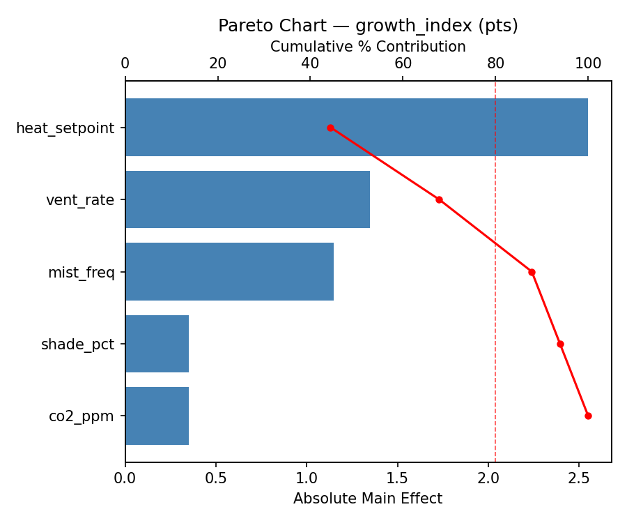
For growth index, the most influential factors were heat setpoint (45.9%), co2 ppm (36.9%), vent rate (11.7%). The best observed value was 8.1 (at vent rate = 5, shade pct = 60, co2 ppm = 400).
For energy cost, the most influential factors were mist freq (40.8%), co2 ppm (28.9%), heat setpoint (19.2%). The best observed value was 6.8 (at vent rate = 30, shade pct = 60, co2 ppm = 1200).
Recommended Next Steps
- Follow up with a response surface design (CCD or Box-Behnken) on the top 3–4 factors to model curvature and find the true optimum.
- Consider whether any fixed factors should be varied in a future study.
- The screening results can guide factor reduction — drop factors contributing less than 5% and re-run with a smaller, more focused design.
Experimental Setup
Factors
| Factor | Low | High | Unit |
|---|
vent_rate | 5 | 30 | ach |
shade_pct | 0 | 60 | % |
co2_ppm | 400 | 1200 | ppm |
heat_setpoint | 15 | 25 | C |
mist_freq | 0 | 12 | per_day |
Fixed: greenhouse_area = 200m2, crop = cucumber
Responses
| Response | Direction | Unit |
|---|
growth_index | ↑ maximize | pts |
energy_cost | ↓ minimize | USD/day |
Configuration
{
"metadata": {
"name": "Greenhouse Climate Control",
"description": "Plackett-Burman screening of ventilation rate, shade cloth, CO2 enrichment, heating setpoint, and misting frequency for plant growth and energy cost"
},
"factors": [
{
"name": "vent_rate",
"levels": [
"5",
"30"
],
"type": "continuous",
"unit": "ach"
},
{
"name": "shade_pct",
"levels": [
"0",
"60"
],
"type": "continuous",
"unit": "%"
},
{
"name": "co2_ppm",
"levels": [
"400",
"1200"
],
"type": "continuous",
"unit": "ppm"
},
{
"name": "heat_setpoint",
"levels": [
"15",
"25"
],
"type": "continuous",
"unit": "C"
},
{
"name": "mist_freq",
"levels": [
"0",
"12"
],
"type": "continuous",
"unit": "per_day"
}
],
"fixed_factors": {
"greenhouse_area": "200m2",
"crop": "cucumber"
},
"responses": [
{
"name": "growth_index",
"optimize": "maximize",
"unit": "pts"
},
{
"name": "energy_cost",
"optimize": "minimize",
"unit": "USD/day"
}
],
"settings": {
"operation": "plackett_burman",
"test_script": "use_cases/105_greenhouse_climate/sim.sh"
}
}
Experimental Matrix
The Plackett-Burman Design produces 8 runs. Each row is one experiment with specific factor settings.
| Run | vent_rate | shade_pct | co2_ppm | heat_setpoint | mist_freq |
|---|
| 1 | 30 | 60 | 1200 | 15 | 0 |
| 2 | 5 | 0 | 1200 | 25 | 0 |
| 3 | 5 | 60 | 400 | 25 | 0 |
| 4 | 30 | 60 | 1200 | 25 | 12 |
| 5 | 5 | 60 | 400 | 15 | 12 |
| 6 | 30 | 0 | 400 | 25 | 12 |
| 7 | 5 | 0 | 1200 | 15 | 12 |
| 8 | 30 | 0 | 400 | 15 | 0 |
Step-by-Step Workflow
1
Preview the design
$ doe info --config use_cases/105_greenhouse_climate/config.json
2
Generate the runner script
$ doe generate --config use_cases/105_greenhouse_climate/config.json \
--output use_cases/105_greenhouse_climate/results/run.sh --seed 42
3
Execute the experiments
$ bash use_cases/105_greenhouse_climate/results/run.sh
4
Analyze results
$ doe analyze --config use_cases/105_greenhouse_climate/config.json
5
Get optimization recommendations
$ doe optimize --config use_cases/105_greenhouse_climate/config.json
6
Multi-objective optimization
With 2 competing responses, use --multi to find the best compromise via Derringer–Suich desirability.
$ doe optimize --config use_cases/105_greenhouse_climate/config.json --multi
7
Generate the HTML report
$ doe report --config use_cases/105_greenhouse_climate/config.json \
--output use_cases/105_greenhouse_climate/results/report.html
Features Exercised
| Feature | Value |
|---|
| Design type | plackett_burman |
| Factor types | continuous (all 5) |
| Arg style | double-dash |
| Responses | 2 (growth_index ↑, energy_cost ↓) |
| Total runs | 8 |
Analysis Results
Generated from actual experiment runs using the DOE Helper Tool.
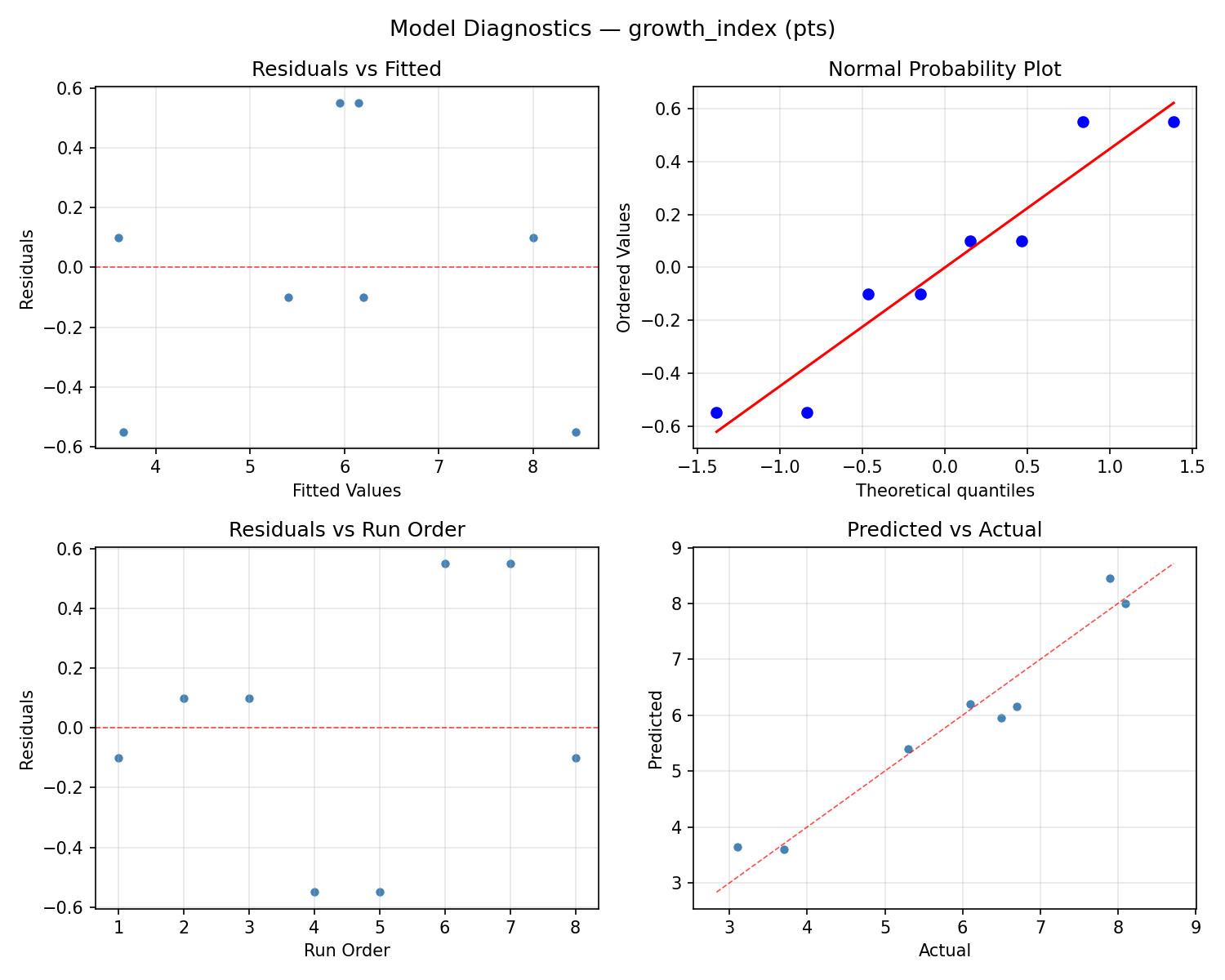
Response: growth_index
Top factors: heat_setpoint (45.9%), co2_ppm (36.9%), vent_rate (11.7%).
ANOVA
| Source | DF | SS | MS | F | p-value |
|---|
| Source | DF | SS | MS | F | p-value |
| vent_rate | 1 | 0.8450 | 0.8450 | 4.507 | 0.0872 |
| shade_pct | 1 | 0.0050 | 0.0050 | 0.027 | 0.8767 |
| co2_ppm | 1 | 8.4050 | 8.4050 | 44.827 | 0.0011 |
| heat_setpoint | 1 | 13.0050 | 13.0050 | 69.360 | 0.0004 |
| mist_freq | 1 | 0.1250 | 0.1250 | 0.667 | 0.4513 |
| vent_rate*shade_pct | 1 | 8.4050 | 8.4050 | 44.827 | 0.0011 |
| vent_rate*co2_ppm | 1 | 0.0050 | 0.0050 | 0.027 | 0.8767 |
| vent_rate*heat_setpoint | 1 | 0.1250 | 0.1250 | 0.667 | 0.4513 |
| vent_rate*mist_freq | 1 | 13.0050 | 13.0050 | 69.360 | 0.0004 |
| shade_pct*co2_ppm | 1 | 0.8450 | 0.8450 | 4.507 | 0.0872 |
| shade_pct*heat_setpoint | 1 | 0.1250 | 0.1250 | 0.667 | 0.4513 |
| shade_pct*mist_freq | 1 | 0.4050 | 0.4050 | 2.160 | 0.2016 |
| co2_ppm*heat_setpoint | 1 | 0.4050 | 0.4050 | 2.160 | 0.2016 |
| co2_ppm*mist_freq | 1 | 0.1250 | 0.1250 | 0.667 | 0.4513 |
| heat_setpoint*mist_freq | 1 | 0.8450 | 0.8450 | 4.507 | 0.0872 |
| Error | (Lenth | PSE) | 5 | 0.9375 | 0.1875 |
| Total | 7 | 22.9150 | 3.2736 | | |
Pareto Chart
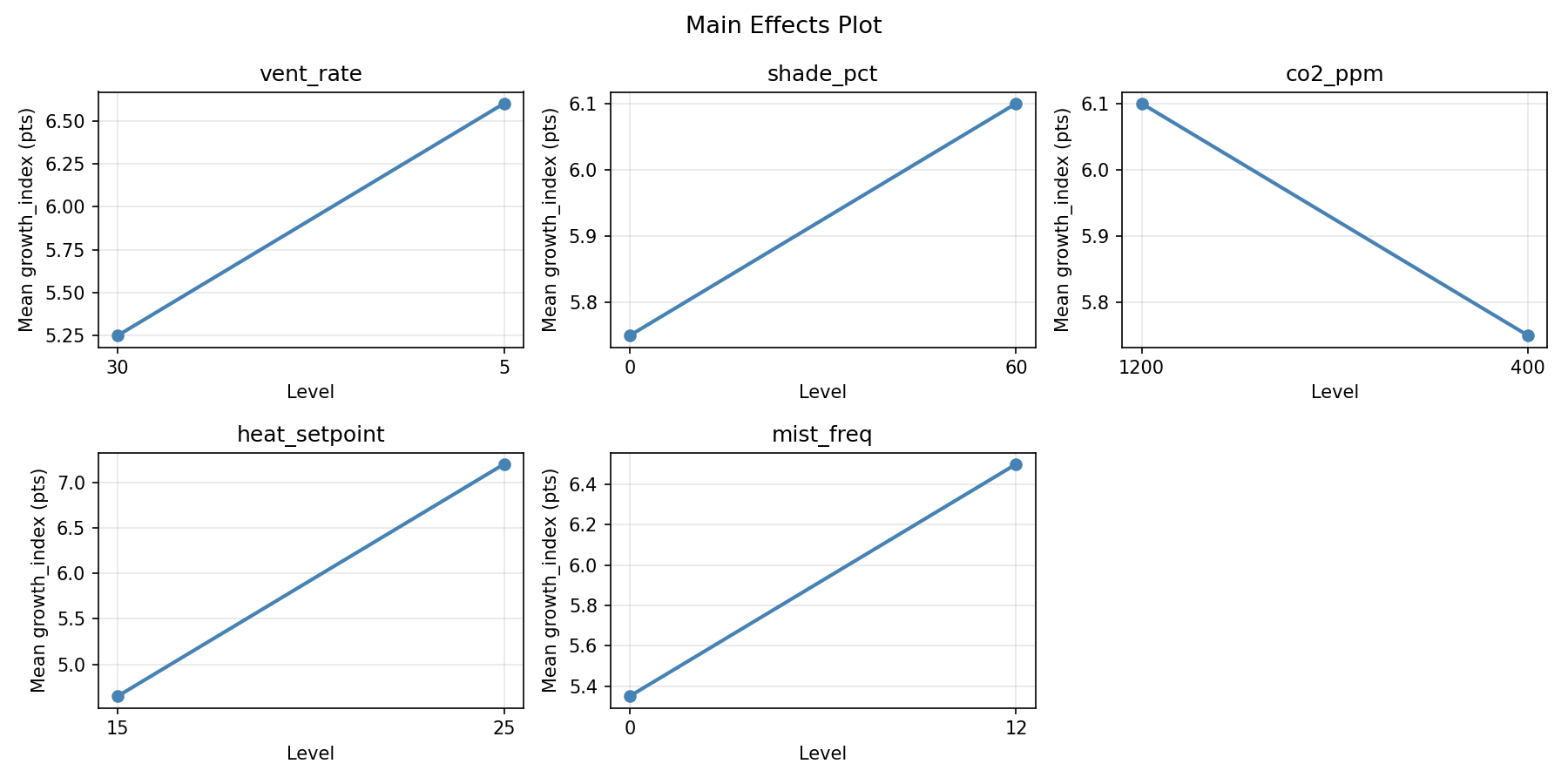
Main Effects Plot
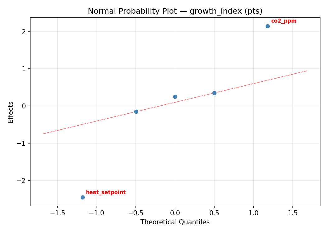
Normal Probability Plot of Effects
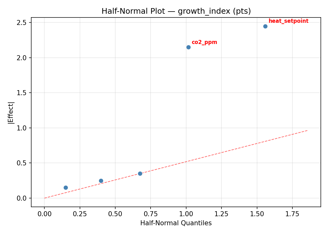
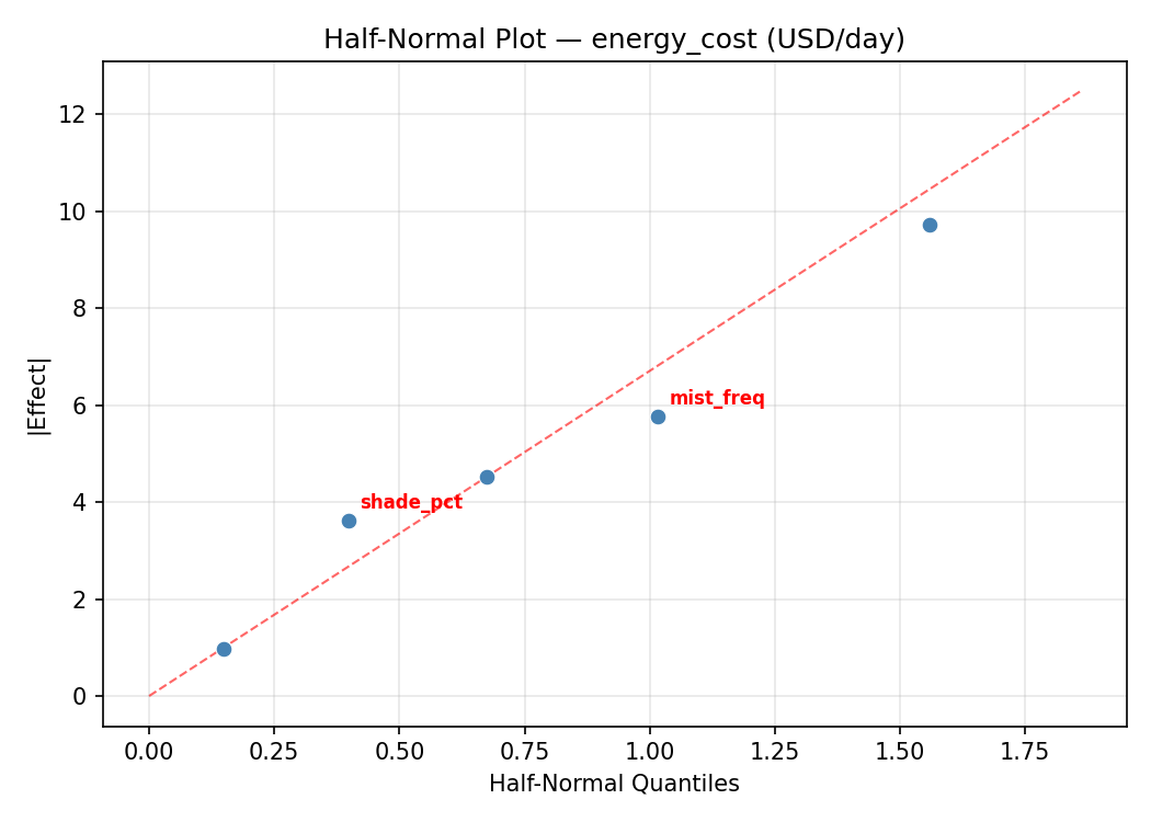
Half-Normal Plot of Effects
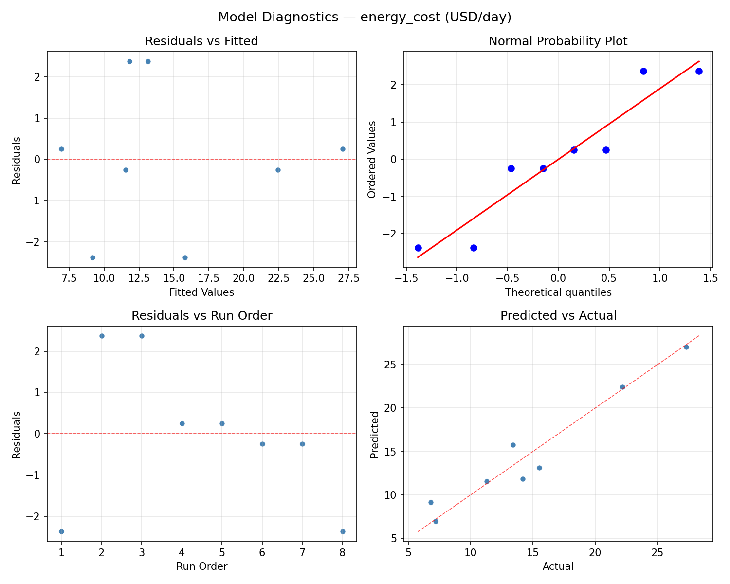
Model Diagnostics
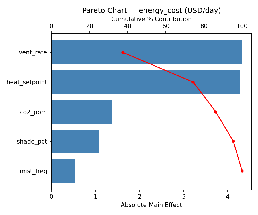
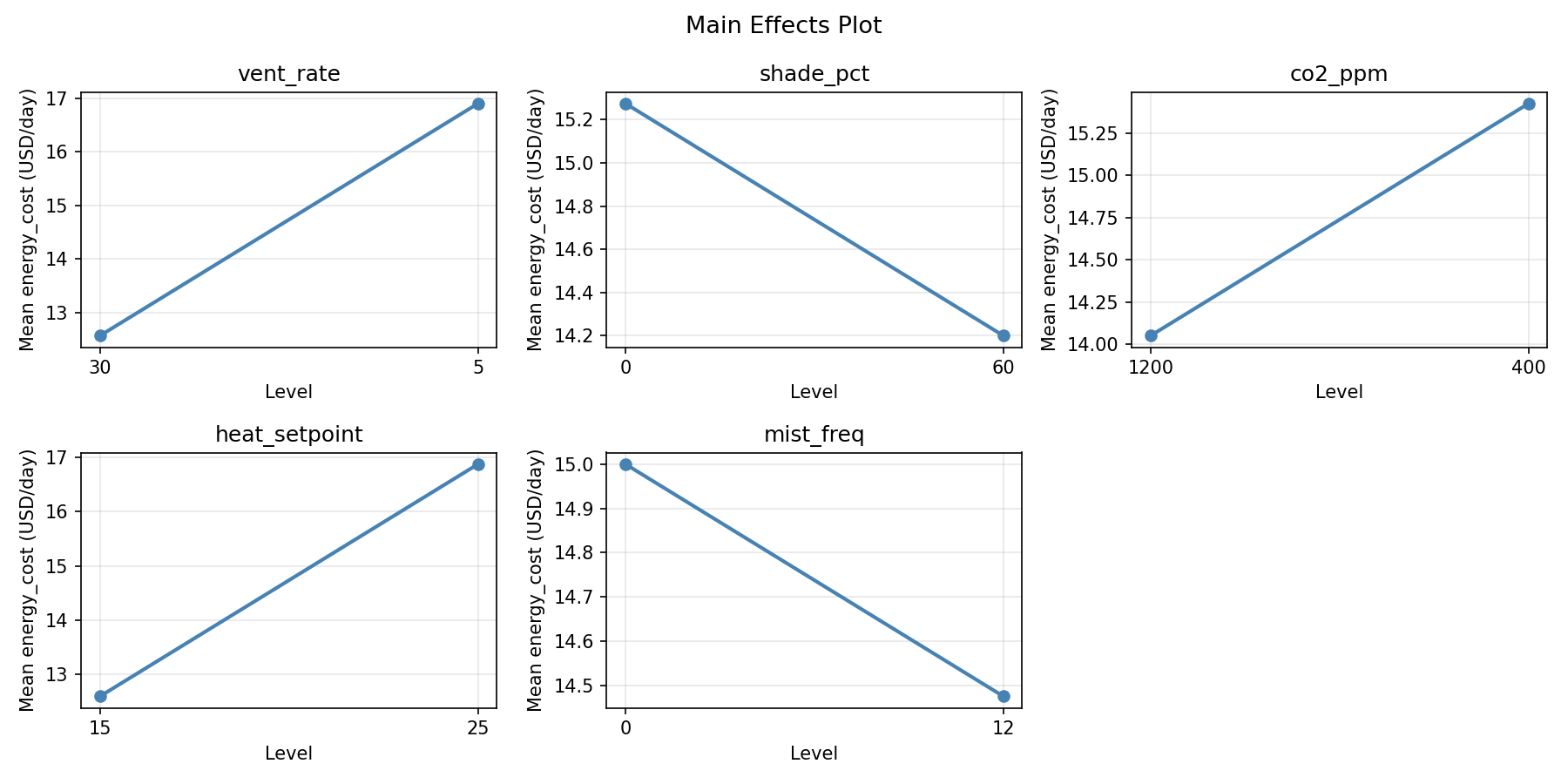
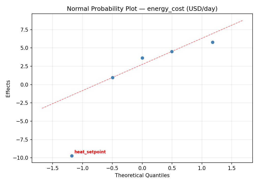
Response: energy_cost
Top factors: mist_freq (40.8%), co2_ppm (28.9%), heat_setpoint (19.2%).
ANOVA
| Source | DF | SS | MS | F | p-value |
|---|
| Source | DF | SS | MS | F | p-value |
| vent_rate | 1 | 9.0312 | 9.0312 | 0.437 | 0.5379 |
| shade_pct | 1 | 0.2113 | 0.2113 | 0.010 | 0.9234 |
| co2_ppm | 1 | 82.5612 | 82.5612 | 3.994 | 0.1021 |
| heat_setpoint | 1 | 36.5513 | 36.5513 | 1.768 | 0.2410 |
| mist_freq | 1 | 164.7112 | 164.7112 | 7.968 | 0.0370 |
| vent_rate*shade_pct | 1 | 82.5613 | 82.5613 | 3.994 | 0.1021 |
| vent_rate*co2_ppm | 1 | 0.2113 | 0.2113 | 0.010 | 0.9234 |
| vent_rate*heat_setpoint | 1 | 164.7113 | 164.7113 | 7.968 | 0.0370 |
| vent_rate*mist_freq | 1 | 36.5513 | 36.5513 | 1.768 | 0.2410 |
| shade_pct*co2_ppm | 1 | 9.0313 | 9.0313 | 0.437 | 0.5379 |
| shade_pct*heat_setpoint | 1 | 40.9513 | 40.9513 | 1.981 | 0.2183 |
| shade_pct*mist_freq | 1 | 13.7813 | 13.7813 | 0.667 | 0.4513 |
| co2_ppm*heat_setpoint | 1 | 13.7812 | 13.7812 | 0.667 | 0.4513 |
| co2_ppm*mist_freq | 1 | 40.9513 | 40.9513 | 1.981 | 0.2183 |
| heat_setpoint*mist_freq | 1 | 9.0313 | 9.0313 | 0.437 | 0.5379 |
| Error | (Lenth | PSE) | 5 | 103.3594 | 20.6719 |
| Total | 7 | 347.7988 | 49.6855 | | |
Pareto Chart
Main Effects Plot
Normal Probability Plot of Effects
Half-Normal Plot of Effects
Model Diagnostics
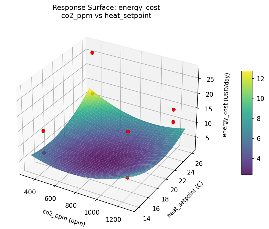
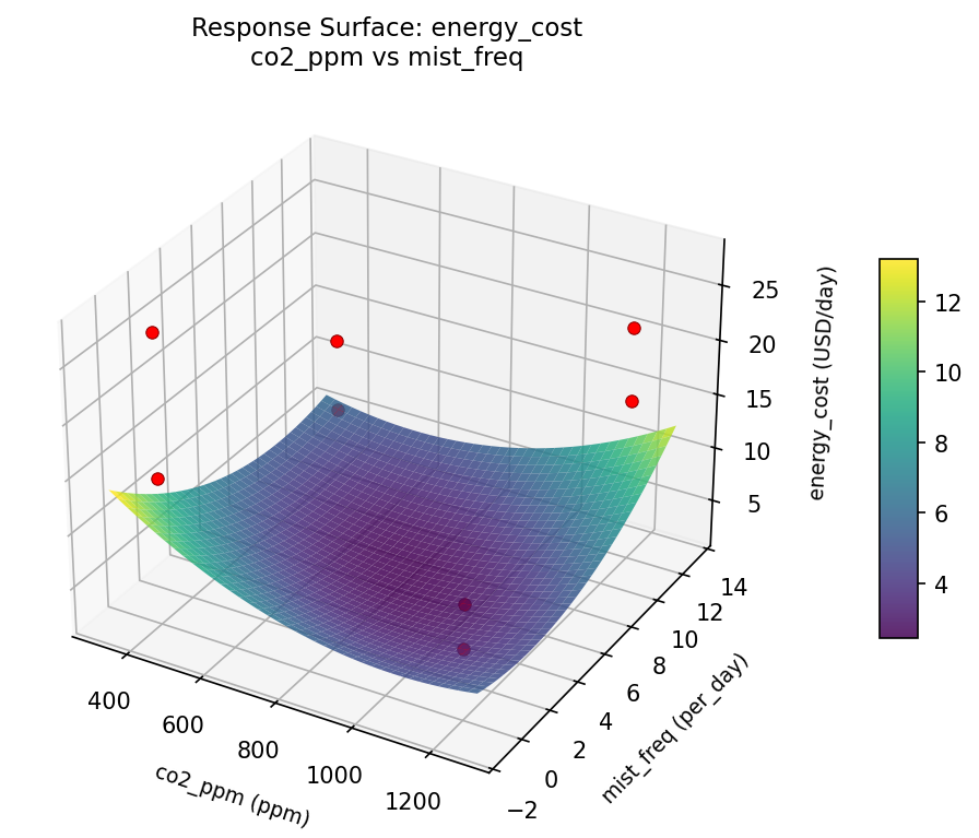
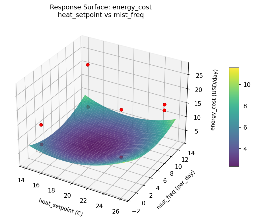
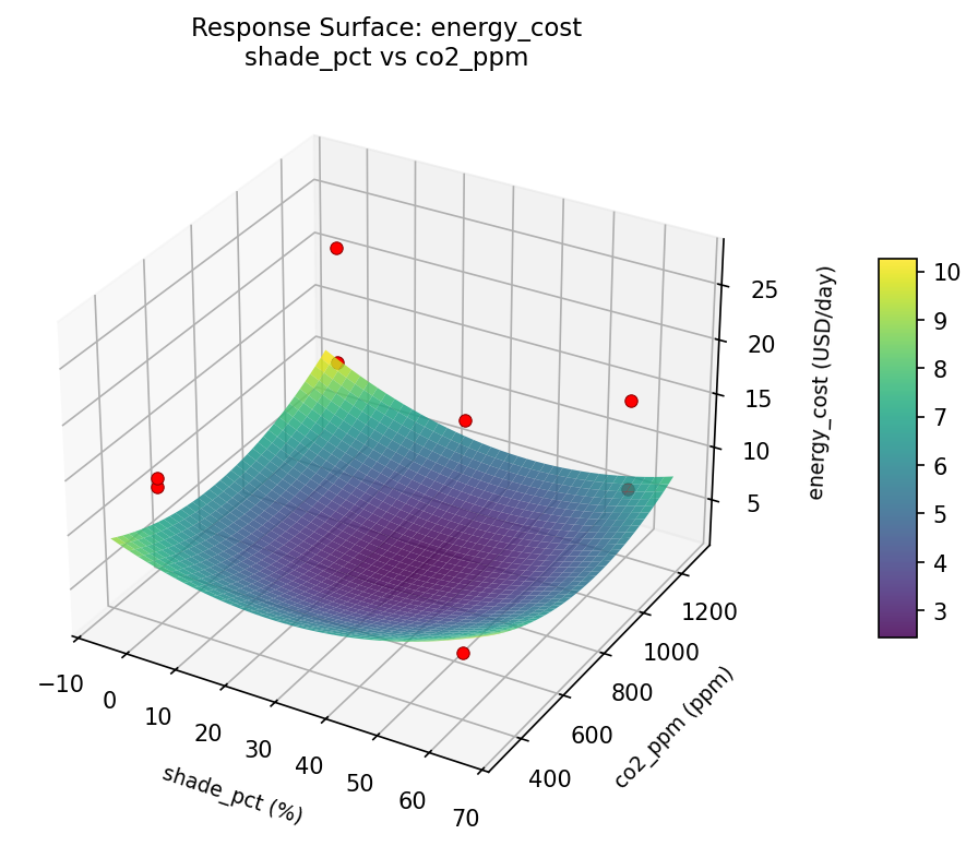
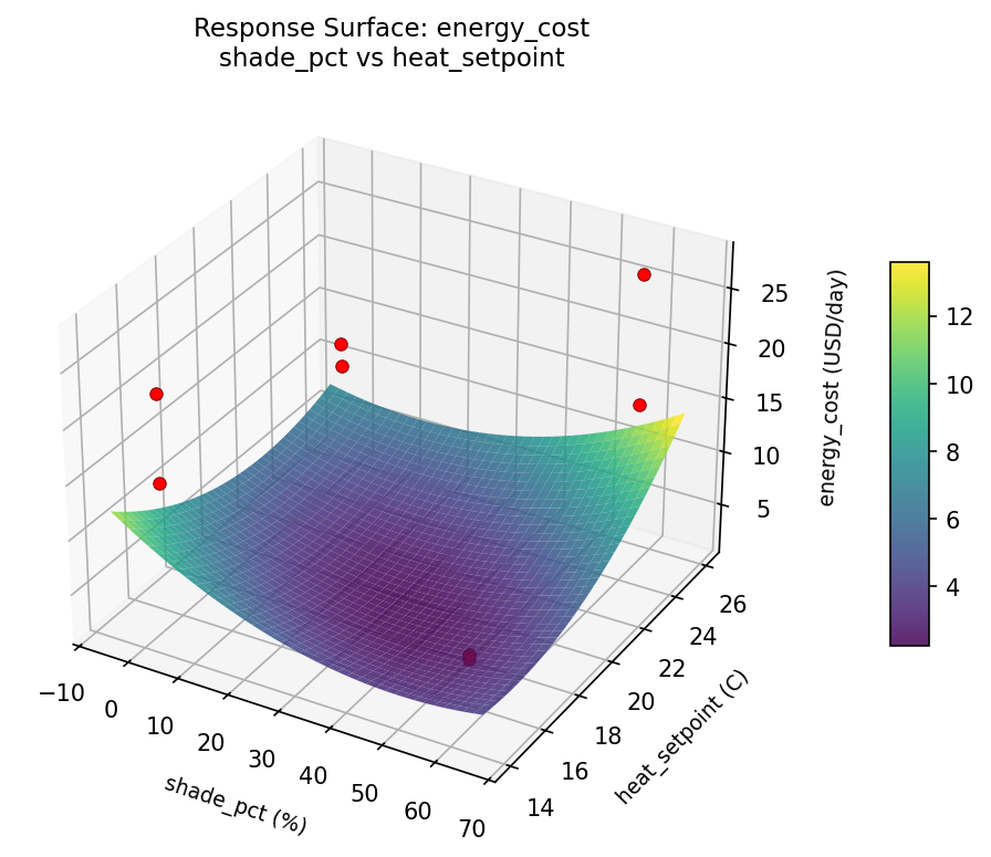
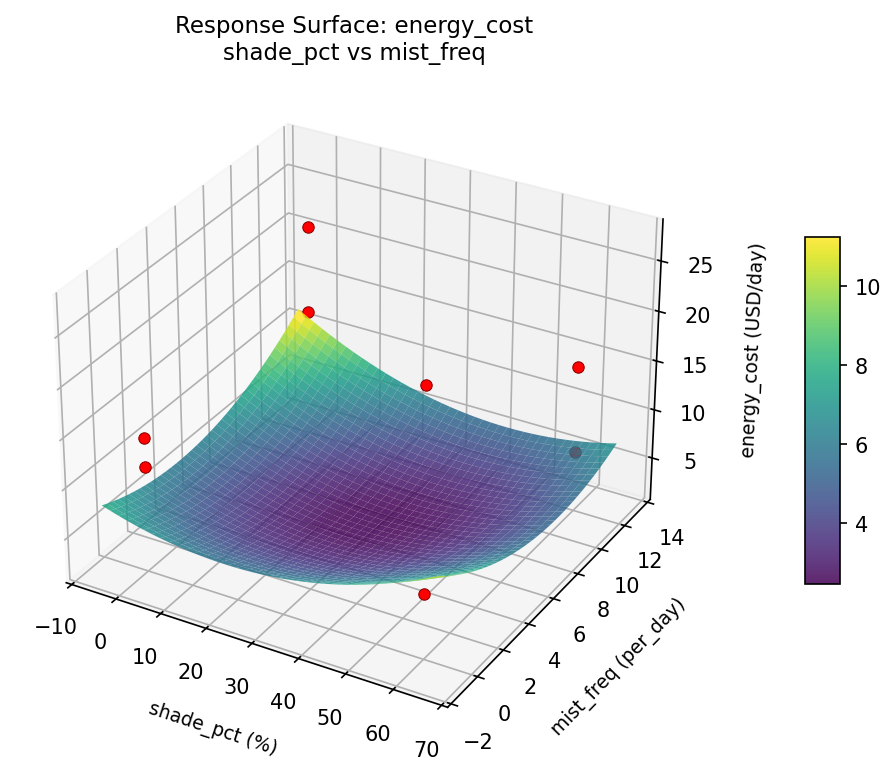
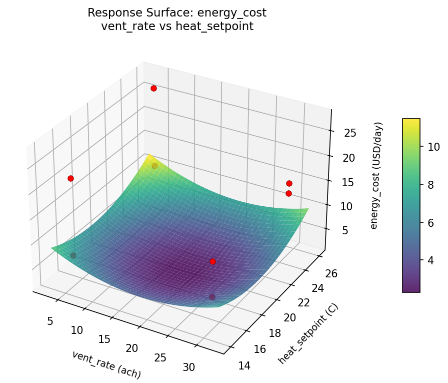
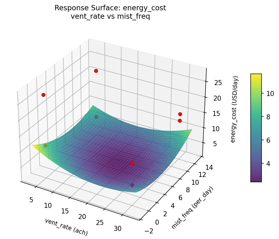
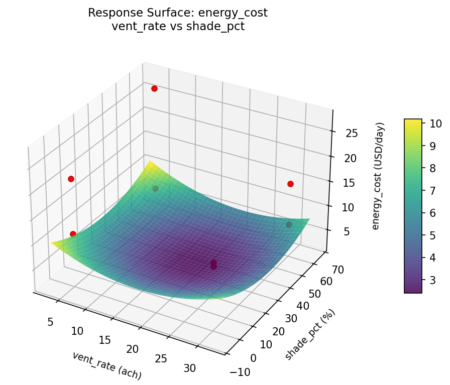
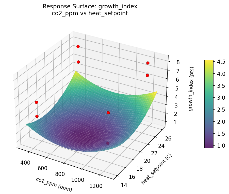
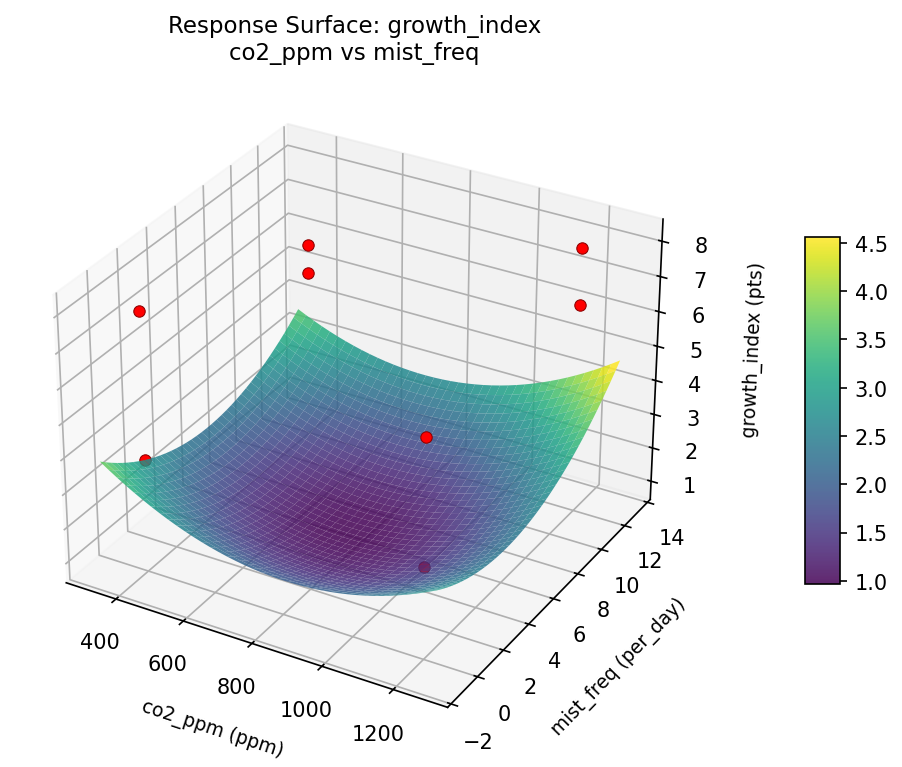
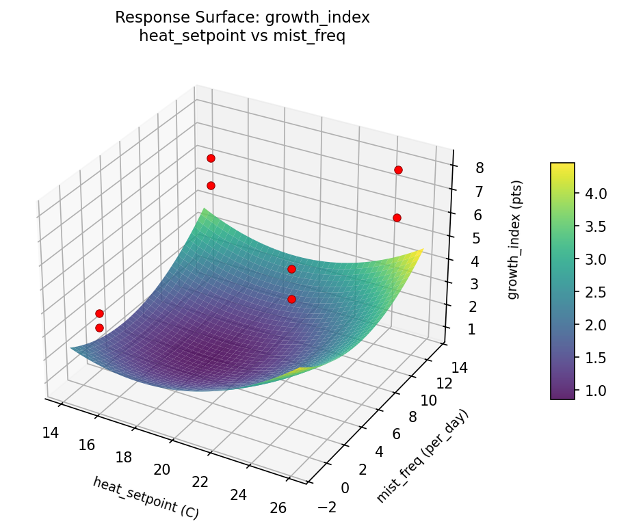
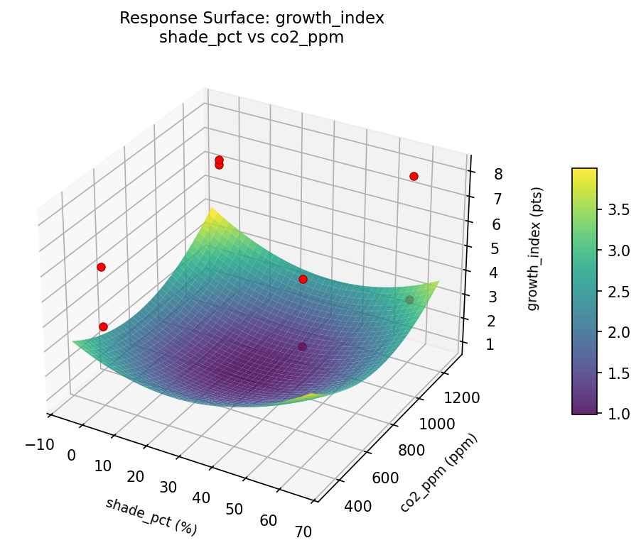
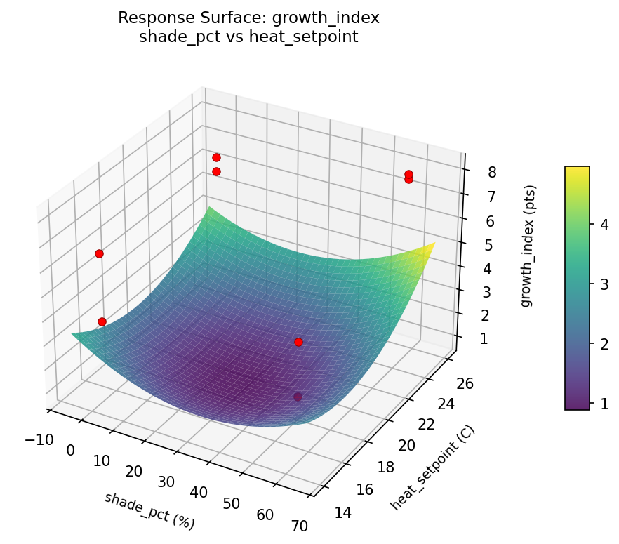
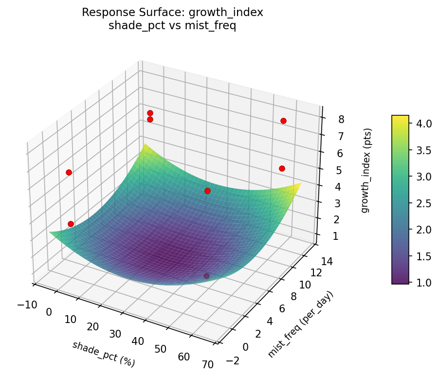
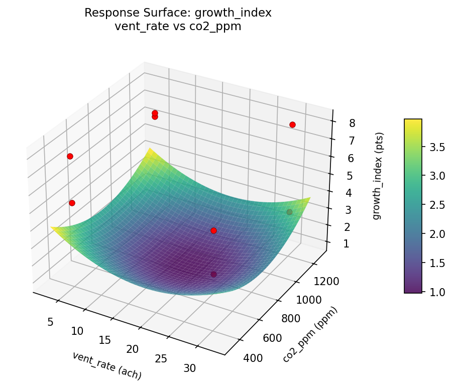
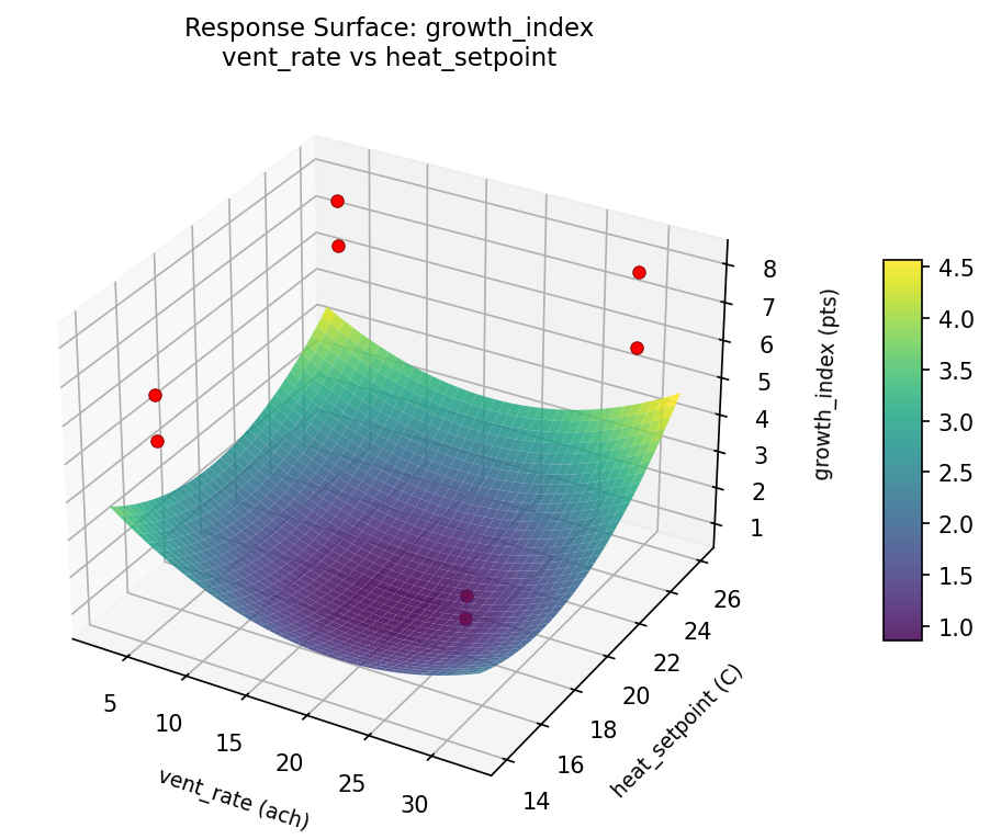
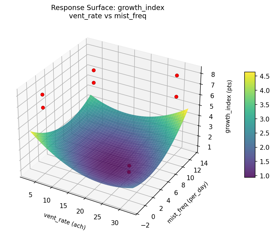
Response Surface Plots
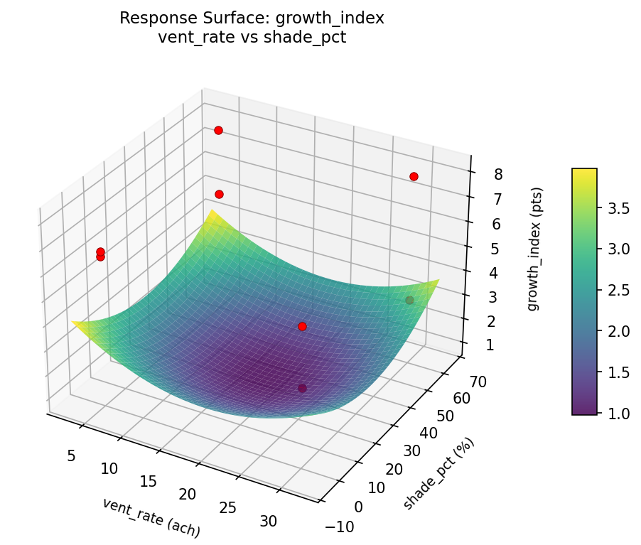
3D surfaces fitted with quadratic RSM. Red dots are observed data points.
energy cost co2 ppm vs heat setpoint
energy cost co2 ppm vs mist freq
energy cost heat setpoint vs mist freq
energy cost shade pct vs co2 ppm
energy cost shade pct vs heat setpoint
energy cost shade pct vs mist freq
energy cost vent rate vs co2 ppm

energy cost vent rate vs heat setpoint
energy cost vent rate vs mist freq
energy cost vent rate vs shade pct
growth index co2 ppm vs heat setpoint
growth index co2 ppm vs mist freq
growth index heat setpoint vs mist freq
growth index shade pct vs co2 ppm
growth index shade pct vs heat setpoint
growth index shade pct vs mist freq
growth index vent rate vs co2 ppm
growth index vent rate vs heat setpoint
growth index vent rate vs mist freq
growth index vent rate vs shade pct
Multi-Objective Optimization
When responses compete, Derringer–Suich desirability finds the best compromise.
Each response is scaled to a 0–1 desirability, then combined via a weighted geometric mean.
Overall Desirability
D = 0.7913
Per-Response Desirability
| Response | Weight | Desirability | Predicted | Dir |
|---|
growth_index |
1.5 |
|
7.93 0.9229 7.93 pts |
↑ |
energy_cost |
1.0 |
|
14.16 0.6281 14.16 USD/day |
↓ |
Recommended Settings
| Factor | Value |
|---|
vent_rate | 6.245 ach |
shade_pct | 50.81 % |
co2_ppm | 1175 ppm |
heat_setpoint | 16.43 C |
mist_freq | 2.143 per_day |
Source: from RSM model prediction
Trade-off Summary
Sacrifice = how much worse than single-objective best.
| Response | Predicted | Best Observed | Sacrifice |
|---|
energy_cost | 14.16 | 6.80 | +7.36 |
Top 3 Runs by Desirability
| Run | D | Factor Settings |
|---|
| #7 | 0.7215 | vent_rate=5, shade_pct=0, co2_ppm=1200, heat_setpoint=15, mist_freq=12 |
| #1 | 0.6183 | vent_rate=5, shade_pct=60, co2_ppm=400, heat_setpoint=15, mist_freq=12 |
Model Quality
| Response | R² | Type |
|---|
energy_cost | 0.8563 | linear |
Full Multi-Objective Output
============================================================
MULTI-OBJECTIVE OPTIMIZATION
Method: Derringer-Suich Desirability Function
============================================================
Overall desirability: D = 0.7913
Response Weight Desirability Predicted Direction
---------------------------------------------------------------------
growth_index 1.5 0.9229 7.93 pts ↑
energy_cost 1.0 0.6281 14.16 USD/day ↓
Recommended settings:
vent_rate = 6.245 ach
shade_pct = 50.81 %
co2_ppm = 1175 ppm
heat_setpoint = 16.43 C
mist_freq = 2.143 per_day
(from RSM model prediction)
Trade-off summary:
growth_index: 7.93 (best observed: 8.10, sacrifice: +0.17)
energy_cost: 14.16 (best observed: 6.80, sacrifice: +7.36)
Model quality:
growth_index: R² = 0.9577 (linear)
energy_cost: R² = 0.8563 (linear)
Top 3 observed runs by overall desirability:
1. Run #2 (D=0.7760): vent_rate=30, shade_pct=60, co2_ppm=1200, heat_setpoint=15, mist_freq=0
2. Run #7 (D=0.7215): vent_rate=5, shade_pct=0, co2_ppm=1200, heat_setpoint=15, mist_freq=12
3. Run #1 (D=0.6183): vent_rate=5, shade_pct=60, co2_ppm=400, heat_setpoint=15, mist_freq=12
Full Analysis Output
=== Main Effects: growth_index ===
Factor Effect Std Error % Contribution
--------------------------------------------------------------
heat_setpoint 2.5500 0.6397 45.9%
co2_ppm 2.0500 0.6397 36.9%
vent_rate -0.6500 0.6397 11.7%
mist_freq -0.2500 0.6397 4.5%
shade_pct -0.0500 0.6397 0.9%
=== ANOVA Table: growth_index ===
Source DF SS MS F p-value
-----------------------------------------------------------------------------
vent_rate 1 0.8450 0.8450 4.507 0.0872
shade_pct 1 0.0050 0.0050 0.027 0.8767
co2_ppm 1 8.4050 8.4050 44.827 0.0011
heat_setpoint 1 13.0050 13.0050 69.360 0.0004
mist_freq 1 0.1250 0.1250 0.667 0.4513
vent_rate*shade_pct 1 8.4050 8.4050 44.827 0.0011
vent_rate*co2_ppm 1 0.0050 0.0050 0.027 0.8767
vent_rate*heat_setpoint 1 0.1250 0.1250 0.667 0.4513
vent_rate*mist_freq 1 13.0050 13.0050 69.360 0.0004
shade_pct*co2_ppm 1 0.8450 0.8450 4.507 0.0872
shade_pct*heat_setpoint 1 0.1250 0.1250 0.667 0.4513
shade_pct*mist_freq 1 0.4050 0.4050 2.160 0.2016
co2_ppm*heat_setpoint 1 0.4050 0.4050 2.160 0.2016
co2_ppm*mist_freq 1 0.1250 0.1250 0.667 0.4513
heat_setpoint*mist_freq 1 0.8450 0.8450 4.507 0.0872
Error (Lenth PSE) 5 0.9375 0.1875
Total 7 22.9150 3.2736
Note: Error estimated using Lenth's pseudo-standard-error (unreplicated design)
=== Interaction Effects: growth_index ===
Factor A Factor B Interaction % Contribution
------------------------------------------------------------------------
vent_rate mist_freq -2.5500 33.6%
vent_rate shade_pct 2.0500 27.0%
shade_pct co2_ppm -0.6500 8.6%
heat_setpoint mist_freq 0.6500 8.6%
shade_pct mist_freq 0.4500 5.9%
co2_ppm heat_setpoint -0.4500 5.9%
vent_rate heat_setpoint 0.2500 3.3%
shade_pct heat_setpoint 0.2500 3.3%
co2_ppm mist_freq -0.2500 3.3%
vent_rate co2_ppm -0.0500 0.7%
=== Summary Statistics: growth_index ===
vent_rate:
Level N Mean Std Min Max
------------------------------------------------------------
30 4 6.2500 1.8430 3.7000 8.1000
5 4 5.6000 1.9900 3.1000 7.9000
shade_pct:
Level N Mean Std Min Max
------------------------------------------------------------
0 4 5.9500 2.0873 3.1000 8.1000
60 4 5.9000 1.8111 3.7000 7.9000
co2_ppm:
Level N Mean Std Min Max
------------------------------------------------------------
1200 4 4.9000 1.7664 3.1000 6.7000
400 4 6.9500 1.3102 5.3000 8.1000
heat_setpoint:
Level N Mean Std Min Max
------------------------------------------------------------
15 4 4.6500 1.5438 3.1000 6.5000
25 4 7.2000 0.9592 6.1000 8.1000
mist_freq:
Level N Mean Std Min Max
------------------------------------------------------------
0 4 6.0500 1.7464 3.7000 7.9000
12 4 5.8000 2.1323 3.1000 8.1000
=== Main Effects: energy_cost ===
Factor Effect Std Error % Contribution
--------------------------------------------------------------
mist_freq -9.0750 2.4921 40.8%
co2_ppm 6.4250 2.4921 28.9%
heat_setpoint 4.2750 2.4921 19.2%
vent_rate -2.1250 2.4921 9.6%
shade_pct 0.3250 2.4921 1.5%
=== ANOVA Table: energy_cost ===
Source DF SS MS F p-value
-----------------------------------------------------------------------------
vent_rate 1 9.0312 9.0312 0.437 0.5379
shade_pct 1 0.2113 0.2113 0.010 0.9234
co2_ppm 1 82.5612 82.5612 3.994 0.1021
heat_setpoint 1 36.5513 36.5513 1.768 0.2410
mist_freq 1 164.7112 164.7112 7.968 0.0370
vent_rate*shade_pct 1 82.5613 82.5613 3.994 0.1021
vent_rate*co2_ppm 1 0.2113 0.2113 0.010 0.9234
vent_rate*heat_setpoint 1 164.7113 164.7113 7.968 0.0370
vent_rate*mist_freq 1 36.5513 36.5513 1.768 0.2410
shade_pct*co2_ppm 1 9.0313 9.0313 0.437 0.5379
shade_pct*heat_setpoint 1 40.9513 40.9513 1.981 0.2183
shade_pct*mist_freq 1 13.7813 13.7813 0.667 0.4513
co2_ppm*heat_setpoint 1 13.7812 13.7812 0.667 0.4513
co2_ppm*mist_freq 1 40.9513 40.9513 1.981 0.2183
heat_setpoint*mist_freq 1 9.0313 9.0313 0.437 0.5379
Error (Lenth PSE) 5 103.3594 20.6719
Total 7 347.7988 49.6855
Note: Error estimated using Lenth's pseudo-standard-error (unreplicated design)
=== Interaction Effects: energy_cost ===
Factor A Factor B Interaction % Contribution
------------------------------------------------------------------------
vent_rate heat_setpoint 9.0750 23.5%
vent_rate shade_pct 6.4250 16.6%
shade_pct heat_setpoint 4.5250 11.7%
co2_ppm mist_freq -4.5250 11.7%
vent_rate mist_freq -4.2750 11.1%
shade_pct mist_freq -2.6250 6.8%
co2_ppm heat_setpoint 2.6250 6.8%
shade_pct co2_ppm -2.1250 5.5%
heat_setpoint mist_freq 2.1250 5.5%
vent_rate co2_ppm 0.3250 0.8%
=== Summary Statistics: energy_cost ===
vent_rate:
Level N Mean Std Min Max
------------------------------------------------------------
30 4 15.8000 4.6137 11.3000 22.2000
5 4 13.6750 9.5727 6.8000 27.3000
shade_pct:
Level N Mean Std Min Max
------------------------------------------------------------
0 4 14.5750 6.1851 7.2000 22.2000
60 4 14.9000 8.8095 6.8000 27.3000
co2_ppm:
Level N Mean Std Min Max
------------------------------------------------------------
1200 4 11.5250 3.1320 7.2000 14.2000
400 4 17.9500 8.8659 6.8000 27.3000
heat_setpoint:
Level N Mean Std Min Max
------------------------------------------------------------
15 4 12.6000 7.2461 6.8000 22.2000
25 4 16.8750 7.1584 11.3000 27.3000
mist_freq:
Level N Mean Std Min Max
------------------------------------------------------------
0 4 19.2750 6.6640 13.4000 27.3000
12 4 10.2000 4.0768 6.8000 15.5000
Optimization Recommendations
=== Optimization: growth_index ===
Direction: maximize
Best observed run: #2
vent_rate = 5
shade_pct = 60
co2_ppm = 400
heat_setpoint = 25
mist_freq = 0
Value: 8.1
RSM Model (linear, R² = 0.9786, Adj R² = 0.9252):
Coefficients:
intercept +5.9250
vent_rate +0.6750
shade_pct +0.6250
co2_ppm -1.2250
heat_setpoint -0.0250
mist_freq -0.6750
Predicted optimum (from linear model, at observed points):
vent_rate = 30
shade_pct = 0
co2_ppm = 400
heat_setpoint = 15
mist_freq = 0
Predicted value: 7.9000
Surface optimum (via L-BFGS-B, linear model):
vent_rate = 30
shade_pct = 60
co2_ppm = 400
heat_setpoint = 15
mist_freq = 0
Predicted value: 9.1500
Model quality: Excellent fit — surface predictions are reliable.
Factor importance:
1. co2_ppm (effect: 2.5, contribution: 38.0%)
2. vent_rate (effect: -1.3, contribution: 20.9%)
3. mist_freq (effect: -1.3, contribution: 20.9%)
4. shade_pct (effect: 1.2, contribution: 19.4%)
5. heat_setpoint (effect: -0.0, contribution: 0.8%)
=== Optimization: energy_cost ===
Direction: minimize
Best observed run: #8
vent_rate = 30
shade_pct = 60
co2_ppm = 1200
heat_setpoint = 25
mist_freq = 12
Value: 6.8
RSM Model (linear, R² = 0.9825, Adj R² = 0.9387):
Coefficients:
intercept +14.7375
vent_rate +2.1625
shade_pct -2.9875
co2_ppm -4.8625
heat_setpoint -0.0625
mist_freq -2.3375
Predicted optimum (from linear model, at observed points):
vent_rate = 30
shade_pct = 0
co2_ppm = 400
heat_setpoint = 15
mist_freq = 0
Predicted value: 27.1500
Surface optimum (via L-BFGS-B, linear model):
vent_rate = 5
shade_pct = 60
co2_ppm = 1200
heat_setpoint = 25
mist_freq = 12
Predicted value: 2.3250
Model quality: Excellent fit — surface predictions are reliable.
Factor importance:
1. co2_ppm (effect: 9.7, contribution: 39.2%)
2. shade_pct (effect: -6.0, contribution: 24.1%)
3. mist_freq (effect: -4.7, contribution: 18.8%)
4. vent_rate (effect: -4.3, contribution: 17.4%)
5. heat_setpoint (effect: -0.1, contribution: 0.5%)