Running Training Plan — DOE Use Case

Summary

This experiment investigates running training plan. Box-Behnken design to maximize VO2max improvement and minimize injury risk by tuning weekly mileage, long run percentage, and interval intensity.

The design varies 3 factors: weekly km (km), ranging from 20 to 60, long run pct (%), ranging from 20 to 40, and interval pct max (%HR_max), ranging from 80 to 100. The goal is to optimize 2 responses: vo2max gain (mL/kg/min) (maximize) and injury risk (%) (minimize). Fixed conditions held constant across all runs include rest days = 2, runner level = intermediate.

A Box-Behnken design was chosen because it efficiently fits quadratic models with 3 continuous factors while avoiding extreme corner combinations — requiring only 15 runs instead of the 8 needed for a full factorial at two levels.

Quadratic response surface models were fitted to capture potential curvature and factor interactions. The RSM contour plots below visualize how pairs of factors jointly affect each response.

Key Findings

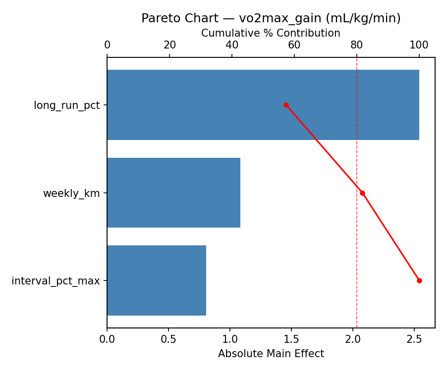
For vo2max gain, the most influential factors were long run pct (53.7%), interval pct max (32.2%), weekly km (14.2%). The best observed value was 5.3 (at weekly km = 20, long run pct = 30, interval pct max = 80).

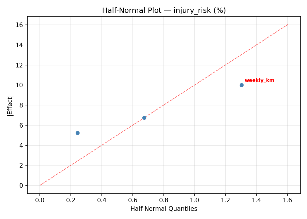
For injury risk, the most influential factors were long run pct (50.1%), interval pct max (39.9%), weekly km (10.0%). The best observed value was 8.0 (at weekly km = 40, long run pct = 40, interval pct max = 100).

Recommended Next Steps

Run confirmation experiments at the predicted optimal settings to validate the model.
Consider whether any fixed factors should be varied in a future study.

Experimental Setup

Factors

Factor	Low	High	Unit
`weekly_km`	20	60	km
`long_run_pct`	20	40	%
`interval_pct_max`	80	100	%HR_max

Fixed: rest_days = 2, runner_level = intermediate

Responses

Response	Direction	Unit
`vo2max_gain`	↑ maximize	mL/kg/min
`injury_risk`	↓ minimize	%

Configuration

use_cases/108_running_performance/config.json

{
  "metadata": {
    "name": "Running Training Plan",
    "description": "Box-Behnken design to maximize VO2max improvement and minimize injury risk by tuning weekly mileage, long run percentage, and interval intensity"
  },
  "factors": [
    {
      "name": "weekly_km",
      "levels": [
        "20",
        "60"
      ],
      "type": "continuous",
      "unit": "km"
    },
    {
      "name": "long_run_pct",
      "levels": [
        "20",
        "40"
      ],
      "type": "continuous",
      "unit": "%"
    },
    {
      "name": "interval_pct_max",
      "levels": [
        "80",
        "100"
      ],
      "type": "continuous",
      "unit": "%HR_max"
    }
  ],
  "fixed_factors": {
    "rest_days": "2",
    "runner_level": "intermediate"
  },
  "responses": [
    {
      "name": "vo2max_gain",
      "optimize": "maximize",
      "unit": "mL/kg/min"
    },
    {
      "name": "injury_risk",
      "optimize": "minimize",
      "unit": "%"
    }
  ],
  "settings": {
    "operation": "box_behnken",
    "test_script": "use_cases/108_running_performance/sim.sh"
  }
}

Experimental Matrix

The Box-Behnken Design produces 15 runs. Each row is one experiment with specific factor settings.

Run	`weekly_km`	`long_run_pct`	`interval_pct_max`
1	40	20	80
2	40	30	90
3	60	30	100
4	60	30	80
5	40	30	90
6	40	30	90
7	20	30	100
8	60	20	90
9	40	20	100
10	60	40	90
11	20	30	80
12	40	40	100
13	20	20	90
14	20	40	90
15	40	40	80

Step-by-Step Workflow

1

Preview the design

Terminal

$ doe info --config use_cases/108_running_performance/config.json

2

Generate the runner script

Terminal

$ doe generate --config use_cases/108_running_performance/config.json \
    --output use_cases/108_running_performance/results/run.sh --seed 42

3

Execute the experiments

Terminal

$ bash use_cases/108_running_performance/results/run.sh

4

Analyze results

Terminal

$ doe analyze --config use_cases/108_running_performance/config.json

5

Get optimization recommendations

Terminal

$ doe optimize --config use_cases/108_running_performance/config.json

6

Multi-objective optimization

With 2 competing responses, use --multi to find the best compromise via Derringer–Suich desirability.

Terminal

$ doe optimize --config use_cases/108_running_performance/config.json --multi

7

Generate the HTML report

Terminal

$ doe report --config use_cases/108_running_performance/config.json \
    --output use_cases/108_running_performance/results/report.html

Features Exercised

Feature	Value
Design type	`box_behnken`
Factor types	`continuous` (all 3)
Arg style	`double-dash`
Responses	2 (vo2max_gain ↑, injury_risk ↓)
Total runs	15

Analysis Results

Generated from actual experiment runs using the DOE Helper Tool.

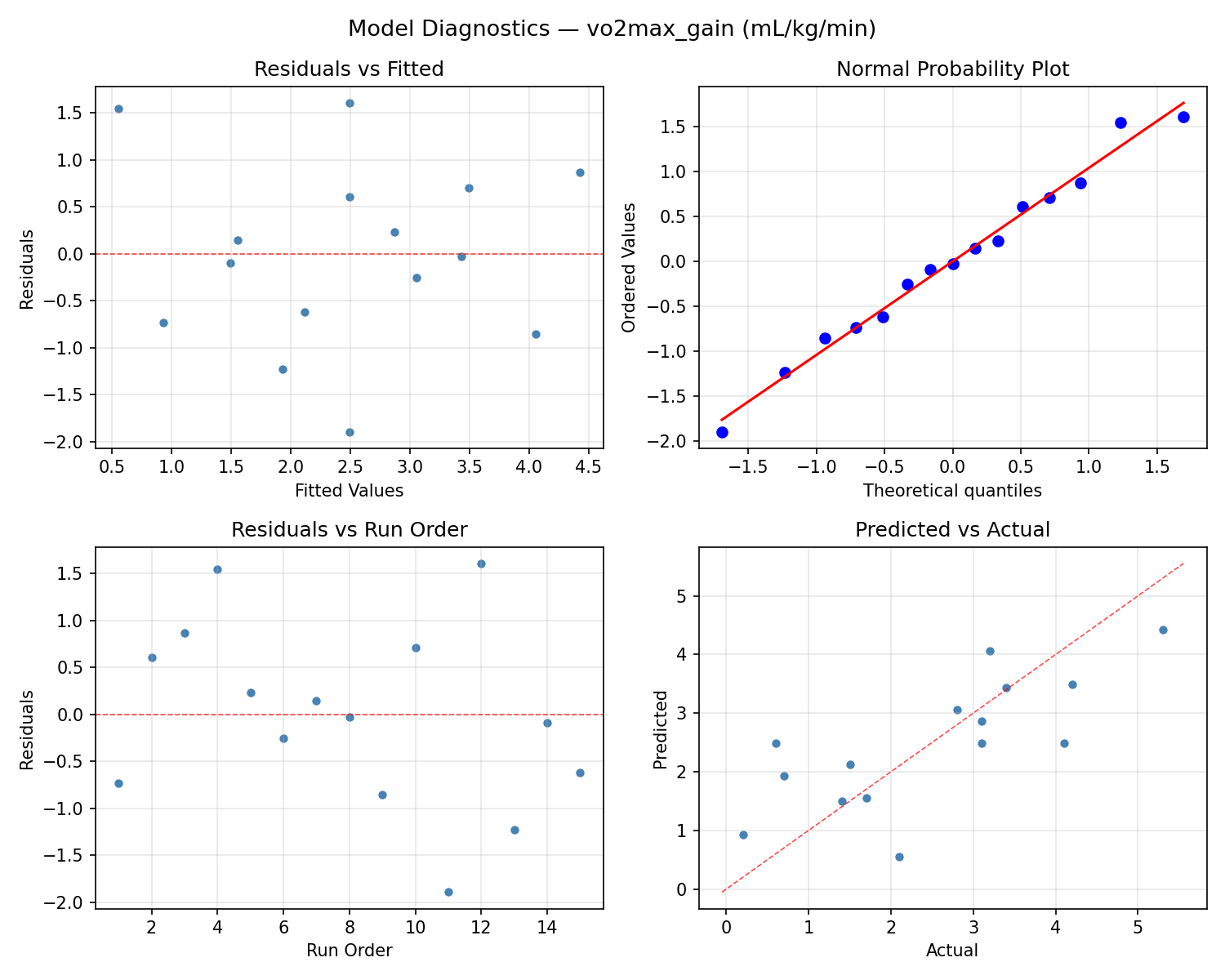
Response: vo2max_gain

Top factors: long_run_pct (53.7%), interval_pct_max (32.2%), weekly_km (14.2%).

ANOVA

Source	DF	SS	MS	F	p-value
Source	DF	SS	MS	F	p-value
weekly_km	2	0.5247	0.2623	0.062	0.9399
long_run_pct	2	6.1718	3.0859	0.734	0.5096
interval_pct_max	2	2.6000	1.3000	0.309	0.7424
Lack	of	Fit	6	12.8461	2.1410
Pure	Error	2	8.4067
Error	8	21.2528	4.2033
Total	14	30.5493	2.1821

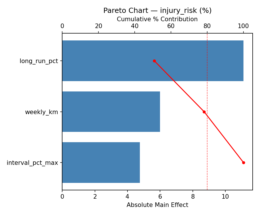
Pareto Chart

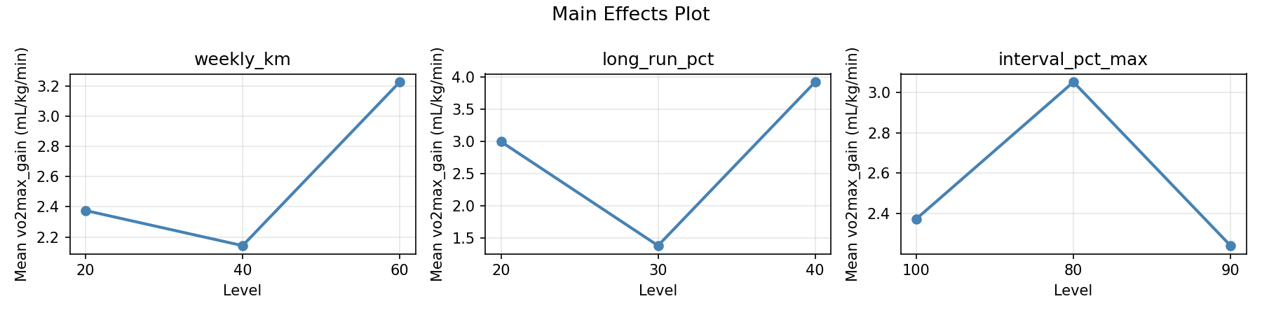
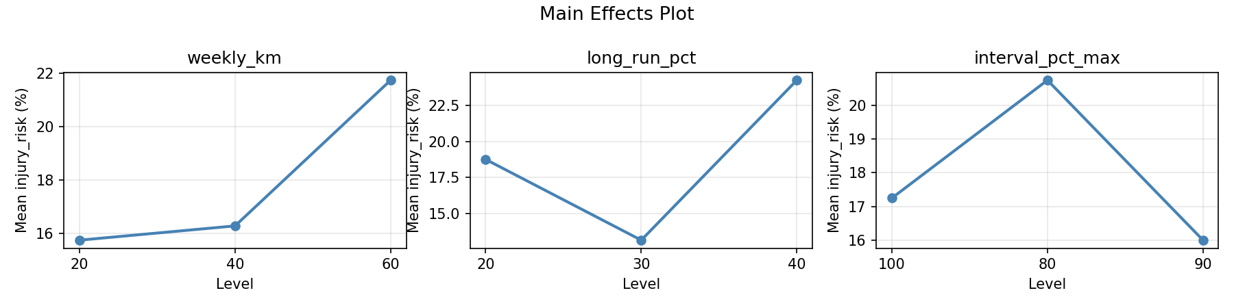
Main Effects Plot

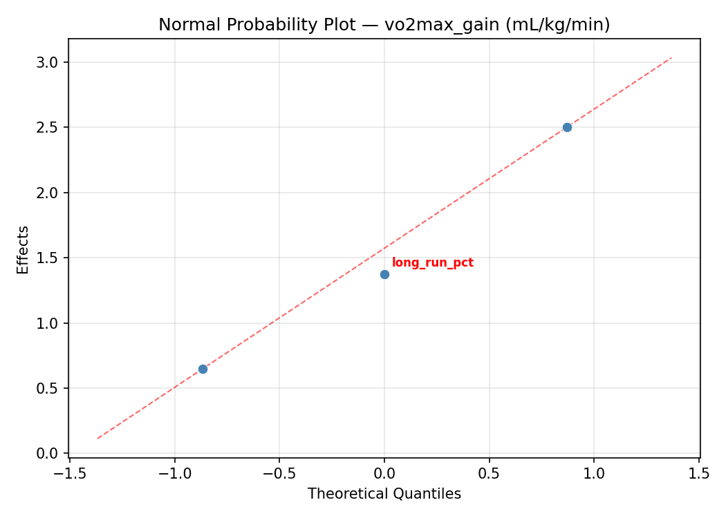
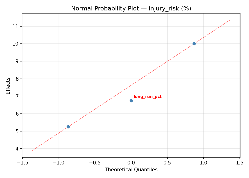
Normal Probability Plot of Effects

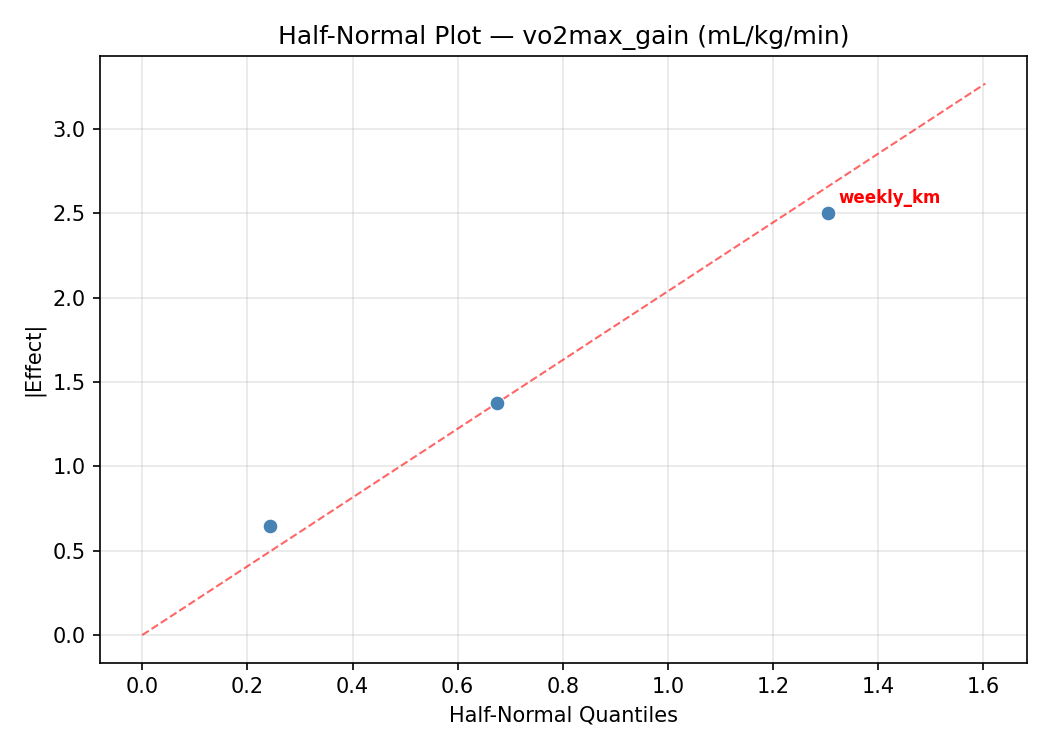
Half-Normal Plot of Effects

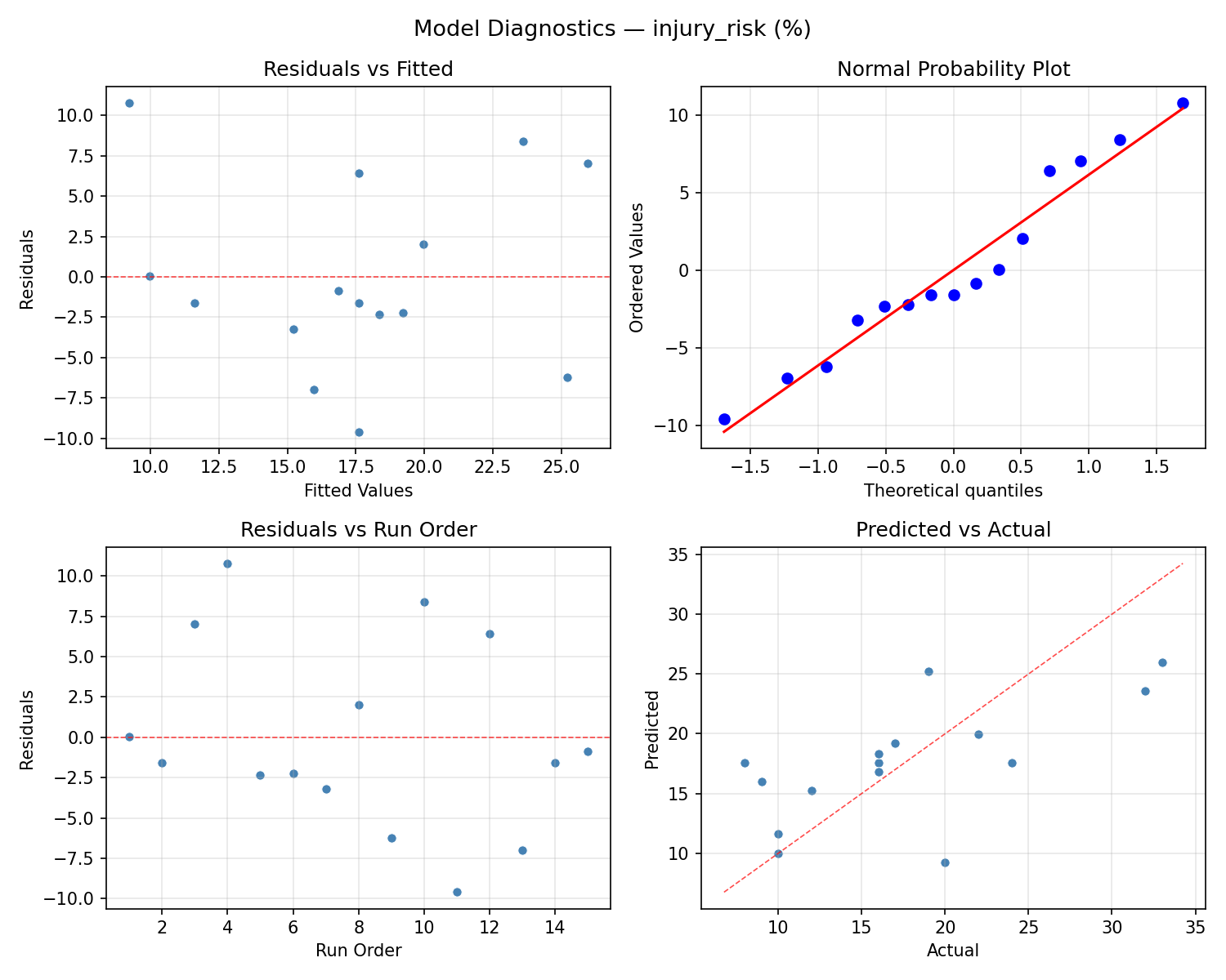
Model Diagnostics

Response: injury_risk

Top factors: long_run_pct (50.1%), interval_pct_max (39.9%), weekly_km (10.0%).

ANOVA

Source	DF	SS	MS	F	p-value
Source	DF	SS	MS	F	p-value
weekly_km	2	6.6000	3.3000	0.022	0.9782
long_run_pct	2	118.6714	59.3357	0.397	0.6847
interval_pct_max	2	90.6714	45.3357	0.304	0.7463
Lack	of	Fit	6	318.9905	53.1651
Pure	Error	2	298.6667
Error	8	617.6571	149.3333
Total	14	833.6000	59.5429

Pareto Chart

Main Effects Plot

Normal Probability Plot of Effects

Half-Normal Plot of Effects

Model Diagnostics

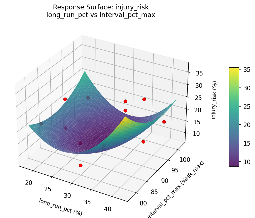
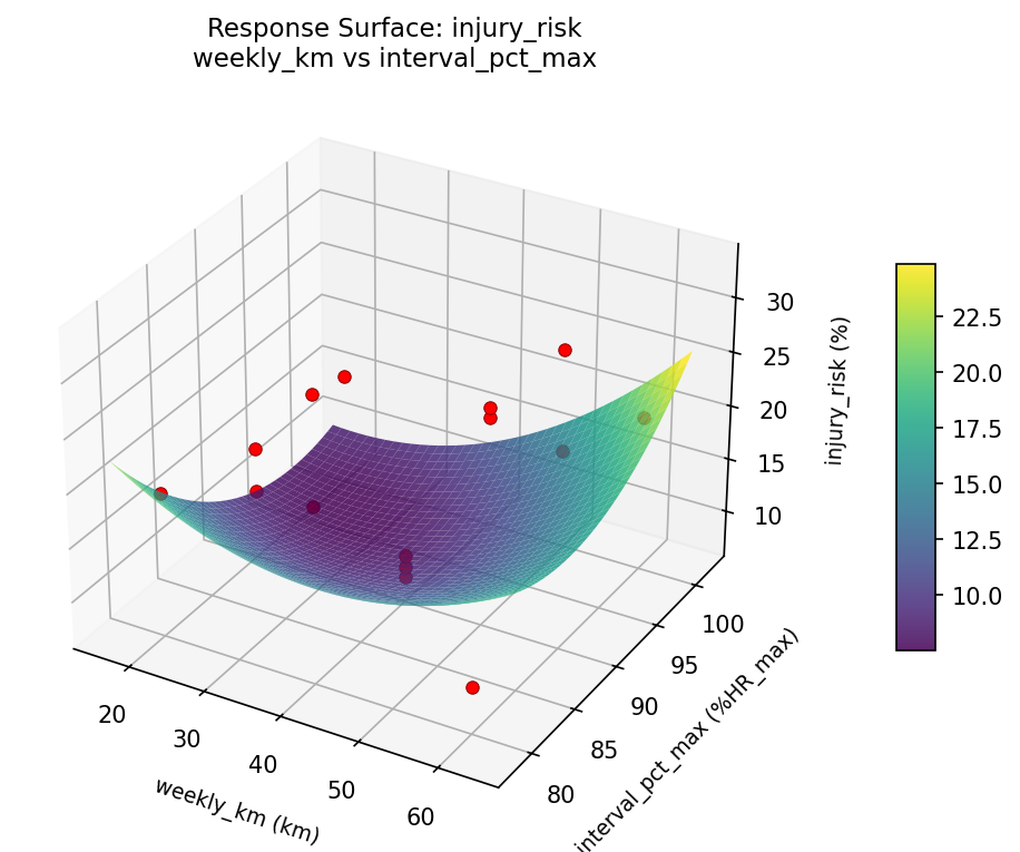
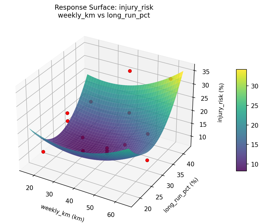
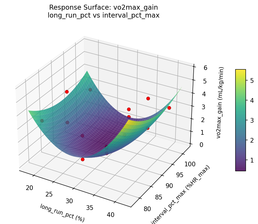
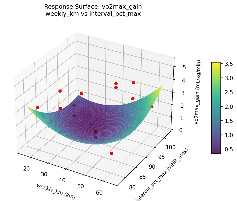
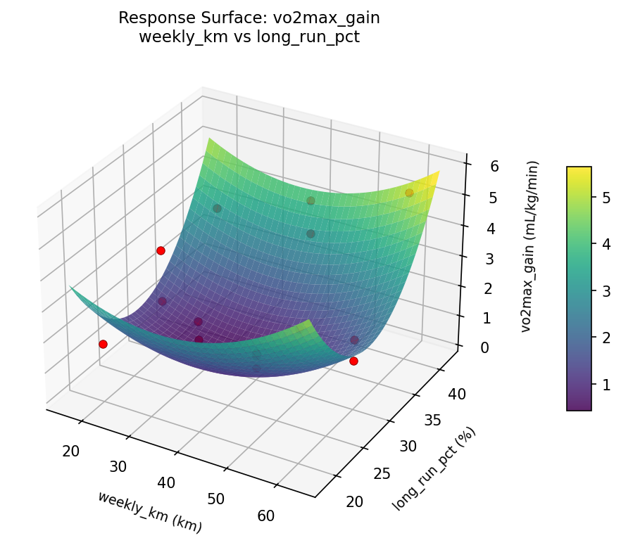
Response Surface Plots

3D surfaces fitted with quadratic RSM. Red dots are observed data points.

injury risk long run pct vs interval pct max

injury risk weekly km vs interval pct max

injury risk weekly km vs long run pct

vo2max gain long run pct vs interval pct max

vo2max gain weekly km vs interval pct max

vo2max gain weekly km vs long run pct

Multi-Objective Optimization

When responses compete, Derringer–Suich desirability finds the best compromise. Each response is scaled to a 0–1 desirability, then combined via a weighted geometric mean.

Overall Desirability

D = 0.6338

Per-Response Desirability

Response	Weight	Desirability	Predicted	Dir
`vo2max_gain`	1.5	0.5978	3.30 0.5978 3.30 mL/kg/min	↑
`injury_risk`	2.0	0.6622	16.04 0.6622 16.04 %	↓

Recommended Settings

Factor	Value
`weekly_km`	36 km
`long_run_pct`	20 %
`interval_pct_max`	100 %HR_max

Source: from RSM model prediction

Trade-off Summary

Sacrifice = how much worse than single-objective best.

Response	Predicted	Best Observed	Sacrifice
`injury_risk`	16.04	8.00	+8.04

Top 3 Runs by Desirability

Run	D	Factor Settings
#5	0.6182	weekly_km=40, long_run_pct=20, interval_pct_max=100
#6	0.5735	weekly_km=60, long_run_pct=30, interval_pct_max=100

Model Quality

Response	R²	Type
`injury_risk`	0.9497	quadratic

Full Multi-Objective Output

doe optimize --multi
============================================================
MULTI-OBJECTIVE OPTIMIZATION
Method: Derringer-Suich Desirability Function
============================================================

Overall desirability: D = 0.6338

Response                  Weight Desirability    Predicted  Direction
---------------------------------------------------------------------
vo2max_gain                  1.5       0.5978        3.30 mL/kg/min   ↑
injury_risk                  2.0       0.6622       16.04 %   ↓

Recommended settings:
  weekly_km = 36 km
  long_run_pct = 20 %
  interval_pct_max = 100 %HR_max
  (from RSM model prediction)

Trade-off summary:
  vo2max_gain: 3.30 (best observed: 5.30, sacrifice: +2.00)
  injury_risk: 16.04 (best observed: 8.00, sacrifice: +8.04)

Model quality:
  vo2max_gain: R² = 0.8881 (quadratic)
  injury_risk: R² = 0.9497 (quadratic)

Top 3 observed runs by overall desirability:
  1. Run #2 (D=0.6182): weekly_km=40, long_run_pct=30, interval_pct_max=90
  2. Run #5 (D=0.6182): weekly_km=40, long_run_pct=20, interval_pct_max=100
  3. Run #6 (D=0.5735): weekly_km=60, long_run_pct=30, interval_pct_max=100

Full Analysis Output

doe analyze
=== Main Effects: vo2max_gain ===
Factor                   Effect    Std Error   % Contribution
--------------------------------------------------------------
long_run_pct             1.6750       0.3814            53.7%
interval_pct_max         1.0036       0.3814            32.2%
weekly_km                0.4429       0.3814            14.2%

=== ANOVA Table: vo2max_gain ===
Source                      DF           SS           MS          F    p-value
-----------------------------------------------------------------------------
weekly_km                    2       0.5247       0.2623      0.062     0.9399
long_run_pct                 2       6.1718       3.0859      0.734     0.5096
interval_pct_max             2       2.6000       1.3000      0.309     0.7424
Lack of Fit                  6      12.8461       2.1410      0.509     0.7792
Pure Error                   2       8.4067       4.2033
Error                        8      21.2528       4.2033
Total                       14      30.5493       2.1821

=== Summary Statistics: vo2max_gain ===

weekly_km:
  Level               N       Mean        Std        Min        Max
  ------------------------------------------------------------
  20                  4     2.8000     0.4967     2.1000     3.2000
  40                  7     2.3571     2.1015     0.2000     5.3000
  60                  4     2.4250     0.9639     1.5000     3.4000

long_run_pct:
  Level               N       Mean        Std        Min        Max
  ------------------------------------------------------------
  20                  4     3.1500     1.8877     0.7000     5.3000
  30                  7     2.7000     1.3102     0.6000     4.2000
  40                  4     1.4750     1.0626     0.2000     2.8000

interval_pct_max:
  Level               N       Mean        Std        Min        Max
  ------------------------------------------------------------
  100                 4     1.8250     1.0243     0.7000     3.1000
  80                  4     2.5750     2.1685     0.2000     5.3000
  90                  7     2.8286     1.3351     0.6000     4.2000

=== Main Effects: injury_risk ===
Factor                   Effect    Std Error   % Contribution
--------------------------------------------------------------
long_run_pct             7.5000       1.9924            50.1%
interval_pct_max         5.9643       1.9924            39.9%
weekly_km                1.5000       1.9924            10.0%

=== ANOVA Table: injury_risk ===
Source                      DF           SS           MS          F    p-value
-----------------------------------------------------------------------------
weekly_km                    2       6.6000       3.3000      0.022     0.9782
long_run_pct                 2     118.6714      59.3357      0.397     0.6847
interval_pct_max             2      90.6714      45.3357      0.304     0.7463
Lack of Fit                  6     318.9905      53.1651      0.356     0.8623
Pure Error                   2     298.6667     149.3333
Error                        8     617.6571     149.3333
Total                       14     833.6000      59.5429

=== Summary Statistics: injury_risk ===

weekly_km:
  Level               N       Mean        Std        Min        Max
  ------------------------------------------------------------
  20                  4    18.0000     1.8257    16.0000    20.0000
  40                  7    18.0000    11.2990     8.0000    33.0000
  60                  4    16.5000     4.1231    12.0000    22.0000

long_run_pct:
  Level               N       Mean        Std        Min        Max
  ------------------------------------------------------------
  20                  4    20.7500     9.8784     9.0000    33.0000
  30                  7    18.2857     7.9522     8.0000    32.0000
  40                  4    13.2500     3.7749    10.0000    17.0000

interval_pct_max:
  Level               N       Mean        Std        Min        Max
  ------------------------------------------------------------
  100                 4    13.7500     5.1881     9.0000    20.0000
  80                  4    17.7500    10.4682    10.0000    33.0000
  90                  7    19.7143     7.4546     8.0000    32.0000

Optimization Recommendations

doe optimize
=== Optimization: vo2max_gain ===
Direction: maximize

Best observed run: #3
  weekly_km = 20
  long_run_pct = 30
  interval_pct_max = 80
  Value: 5.3

RSM Model (linear, R² = 0.1189, Adj R² = -0.1214):
  Coefficients:
    intercept                      +2.4933
    weekly_km                      -0.5875
    long_run_pct                   -0.1375
    interval_pct_max               +0.3000

RSM Model (quadratic, R² = 0.5858, Adj R² = -0.1598):
  Coefficients:
    intercept                      +2.4667
    weekly_km                      -0.5875
    long_run_pct                   -0.1375
    interval_pct_max               +0.3000
    weekly_km*long_run_pct         -0.3500
    weekly_km*interval_pct_max     +1.1250
    long_run_pct*interval_pct_max  -0.3250
    weekly_km^2                    +1.1917
    long_run_pct^2                 -0.5583
    interval_pct_max^2             -0.5833

  Curvature analysis:
    weekly_km                      coef=+1.1917  convex (has a minimum)
    interval_pct_max               coef=-0.5833  concave (has a maximum)
    long_run_pct                   coef=-0.5583  concave (has a maximum)

  Notable interactions:
    weekly_km*interval_pct_max     coef=+1.1250  (synergistic)
    weekly_km*long_run_pct         coef=-0.3500  (antagonistic)
    long_run_pct*interval_pct_max  coef=-0.3250  (antagonistic)

  Predicted optimum (from linear model, at observed points):
    weekly_km = 20
    long_run_pct = 30
    interval_pct_max = 100
    Predicted value: 3.3808

  Surface optimum (via L-BFGS-B, linear model):
    weekly_km = 20
    long_run_pct = 20
    interval_pct_max = 100
    Predicted value: 3.5183

  Model quality: Weak fit — consider adding center points or using a different design.

Factor importance:
  1. weekly_km  (effect: 1.9, contribution: 52.7%)
  2. interval_pct_max  (effect: 0.9, contribution: 26.3%)
  3. long_run_pct  (effect: 0.7, contribution: 21.0%)

=== Optimization: injury_risk ===
Direction: minimize

Best observed run: #11
  weekly_km = 40
  long_run_pct = 40
  interval_pct_max = 100
  Value: 8.0

RSM Model (linear, R² = 0.1551, Adj R² = -0.0754):
  Coefficients:
    intercept                      +17.6000
    weekly_km                      -4.0000
    long_run_pct                   +0.1250
    interval_pct_max               -0.3750

RSM Model (quadratic, R² = 0.5972, Adj R² = -0.1278):
  Coefficients:
    intercept                      +20.0000
    weekly_km                      -4.0000
    long_run_pct                   +0.1250
    interval_pct_max               -0.3750
    weekly_km*long_run_pct         +0.2500
    weekly_km*interval_pct_max     +5.2500
    long_run_pct*interval_pct_max  -2.0000
    weekly_km^2                    +4.5000
    long_run_pct^2                 -3.7500
    interval_pct_max^2             -5.2500

  Curvature analysis:
    interval_pct_max               coef=-5.2500  concave (has a maximum)
    weekly_km                      coef=+4.5000  convex (has a minimum)
    long_run_pct                   coef=-3.7500  concave (has a maximum)

  Notable interactions:
    weekly_km*interval_pct_max     coef=+5.2500  (synergistic)
    long_run_pct*interval_pct_max  coef=-2.0000  (antagonistic)

  Predicted optimum (from linear model, at observed points):
    weekly_km = 20
    long_run_pct = 30
    interval_pct_max = 80
    Predicted value: 21.9750

  Surface optimum (via L-BFGS-B, linear model):
    weekly_km = 60
    long_run_pct = 20
    interval_pct_max = 100
    Predicted value: 13.1000

  Model quality: Weak fit — consider adding center points or using a different design.

Factor importance:
  1. weekly_km  (effect: 9.1, contribution: 49.0%)
  2. interval_pct_max  (effect: 5.7, contribution: 30.5%)
  3. long_run_pct  (effect: 3.8, contribution: 20.5%)

Run	`weekly_km`	`long_run_pct`	`interval_pct_max`
1	40	20	80
2	40	30	90
3	60	30	100
4	60	30	80
5	40	30	90
6	40	30	90
7	20	30	100
8	60	20	90
9	40	20	100
10	60	40	90
11	20	30	80
12	40	40	100
13	20	20	90
14	20	40	90
15	40	40	80

Run	`weekly_km`	`long_run_pct`	`interval_pct_max`
1	40	20	80
2	40	30	90
3	60	30	100
4	60	30	80
5	40	30	90
6	40	30	90
7	20	30	100
8	60	20	90
9	40	20	100
10	60	40	90
11	20	30	80
12	40	40	100
13	20	20	90
14	20	40	90
15	40	40	80

Run	`weekly_km`	`long_run_pct`	`interval_pct_max`
1	40	20	80
2	40	30	90
3	60	30	100
4	60	30	80
5	40	30	90
6	40	30	90
7	20	30	100
8	60	20	90
9	40	20	100
10	60	40	90
11	20	30	80
12	40	40	100
13	20	20	90
14	20	40	90
15	40	40	80