Summary
This experiment investigates strength training program. Full factorial of sets, reps, rest period, and training frequency to maximize strength gain and minimize fatigue score.
The design varies 4 factors: sets (sets), ranging from 3 to 6, reps (reps), ranging from 3 to 12, rest sec (sec), ranging from 60 to 180, and freq per week (days/wk), ranging from 2 to 5. The goal is to optimize 2 responses: strength gain (%) (maximize) and fatigue score (pts) (minimize). Fixed conditions held constant across all runs include exercise = barbell_squat, trainee level = intermediate.
A full factorial design was used to explore all 16 possible combinations of the 4 factors at two levels. This guarantees that every main effect and interaction can be estimated independently, at the cost of a larger experiment (16 runs).
Quadratic response surface models were fitted to capture potential curvature and factor interactions. The RSM contour plots below visualize how pairs of factors jointly affect each response.
Key Findings
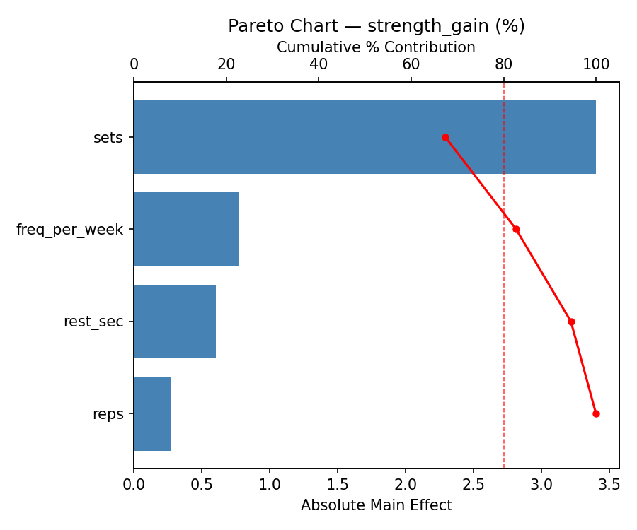
For strength gain, the most influential factors were sets (76.2%), reps (10.2%), freq per week (10.2%). The best observed value was 14.1 (at sets = 6, reps = 12, rest sec = 60).
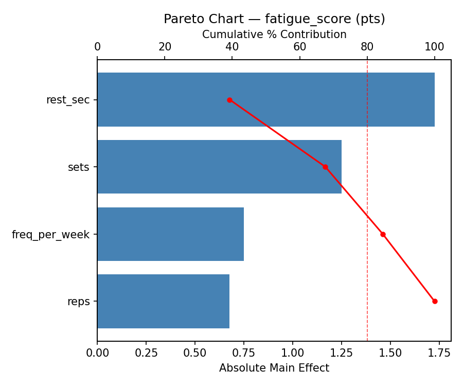
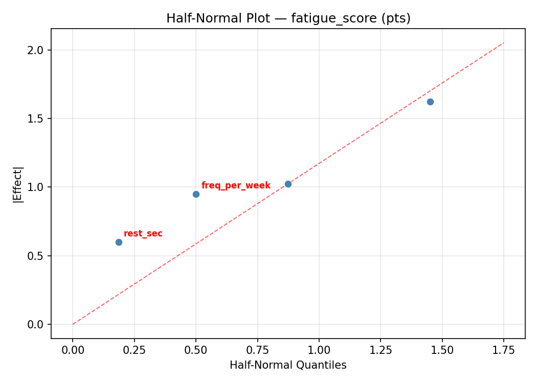
For fatigue score, the most influential factors were sets (70.8%), reps (19.0%), freq per week (6.7%). The best observed value was 1.0 (at sets = 3, reps = 12, rest sec = 60).
Recommended Next Steps
- Consider whether any fixed factors should be varied in a future study.
Experimental Setup
Factors
| Factor | Low | High | Unit |
|---|
sets | 3 | 6 | sets |
reps | 3 | 12 | reps |
rest_sec | 60 | 180 | sec |
freq_per_week | 2 | 5 | days/wk |
Fixed: exercise = barbell_squat, trainee_level = intermediate
Responses
| Response | Direction | Unit |
|---|
strength_gain | ↑ maximize | % |
fatigue_score | ↓ minimize | pts |
Configuration
{
"metadata": {
"name": "Strength Training Program",
"description": "Full factorial of sets, reps, rest period, and training frequency to maximize strength gain and minimize fatigue score"
},
"factors": [
{
"name": "sets",
"levels": [
"3",
"6"
],
"type": "continuous",
"unit": "sets"
},
{
"name": "reps",
"levels": [
"3",
"12"
],
"type": "continuous",
"unit": "reps"
},
{
"name": "rest_sec",
"levels": [
"60",
"180"
],
"type": "continuous",
"unit": "sec"
},
{
"name": "freq_per_week",
"levels": [
"2",
"5"
],
"type": "continuous",
"unit": "days/wk"
}
],
"fixed_factors": {
"exercise": "barbell_squat",
"trainee_level": "intermediate"
},
"responses": [
{
"name": "strength_gain",
"optimize": "maximize",
"unit": "%"
},
{
"name": "fatigue_score",
"optimize": "minimize",
"unit": "pts"
}
],
"settings": {
"operation": "full_factorial",
"test_script": "use_cases/109_strength_training/sim.sh"
}
}
Experimental Matrix
The Full Factorial Design produces 16 runs. Each row is one experiment with specific factor settings.
| Run | sets | reps | rest_sec | freq_per_week |
|---|
| 1 | 3 | 12 | 180 | 5 |
| 2 | 6 | 3 | 60 | 5 |
| 3 | 3 | 12 | 60 | 5 |
| 4 | 3 | 12 | 180 | 2 |
| 5 | 6 | 12 | 180 | 2 |
| 6 | 6 | 3 | 180 | 2 |
| 7 | 6 | 12 | 60 | 2 |
| 8 | 6 | 3 | 60 | 2 |
| 9 | 3 | 3 | 60 | 5 |
| 10 | 3 | 3 | 180 | 2 |
| 11 | 6 | 12 | 60 | 5 |
| 12 | 6 | 12 | 180 | 5 |
| 13 | 3 | 12 | 60 | 2 |
| 14 | 6 | 3 | 180 | 5 |
| 15 | 3 | 3 | 60 | 2 |
| 16 | 3 | 3 | 180 | 5 |
Step-by-Step Workflow
1
Preview the design
$ doe info --config use_cases/109_strength_training/config.json
2
Generate the runner script
$ doe generate --config use_cases/109_strength_training/config.json \
--output use_cases/109_strength_training/results/run.sh --seed 42
3
Execute the experiments
$ bash use_cases/109_strength_training/results/run.sh
4
Analyze results
$ doe analyze --config use_cases/109_strength_training/config.json
5
Get optimization recommendations
$ doe optimize --config use_cases/109_strength_training/config.json
6
Multi-objective optimization
With 2 competing responses, use --multi to find the best compromise via Derringer–Suich desirability.
$ doe optimize --config use_cases/109_strength_training/config.json --multi
7
Generate the HTML report
$ doe report --config use_cases/109_strength_training/config.json \
--output use_cases/109_strength_training/results/report.html
Features Exercised
| Feature | Value |
|---|
| Design type | full_factorial |
| Factor types | continuous (all 4) |
| Arg style | double-dash |
| Responses | 2 (strength_gain ↑, fatigue_score ↓) |
| Total runs | 16 |
Analysis Results
Generated from actual experiment runs using the DOE Helper Tool.
Response: strength_gain
Top factors: sets (76.2%), reps (10.2%), freq_per_week (10.2%).
ANOVA
| Source | DF | SS | MS | F | p-value |
|---|
| Source | DF | SS | MS | F | p-value |
| sets | 1 | 31.3600 | 31.3600 | 1.928 | 0.2236 |
| reps | 1 | 0.5625 | 0.5625 | 0.035 | 0.8598 |
| rest_sec | 1 | 0.0625 | 0.0625 | 0.004 | 0.9530 |
| freq_per_week | 1 | 0.5625 | 0.5625 | 0.035 | 0.8598 |
| sets*reps | 1 | 3.4225 | 3.4225 | 0.210 | 0.6657 |
| sets*rest_sec | 1 | 6.5025 | 6.5025 | 0.400 | 0.5550 |
| sets*freq_per_week | 1 | 1.8225 | 1.8225 | 0.112 | 0.7514 |
| reps*rest_sec | 1 | 1.6900 | 1.6900 | 0.104 | 0.7602 |
| reps*freq_per_week | 1 | 32.4900 | 32.4900 | 1.998 | 0.2167 |
| rest_sec*freq_per_week | 1 | 0.2500 | 0.2500 | 0.015 | 0.9062 |
| Error | 5 | 81.3150 | 16.2630 | | |
| Total | 15 | 160.0400 | 10.6693 | | |
Pareto Chart
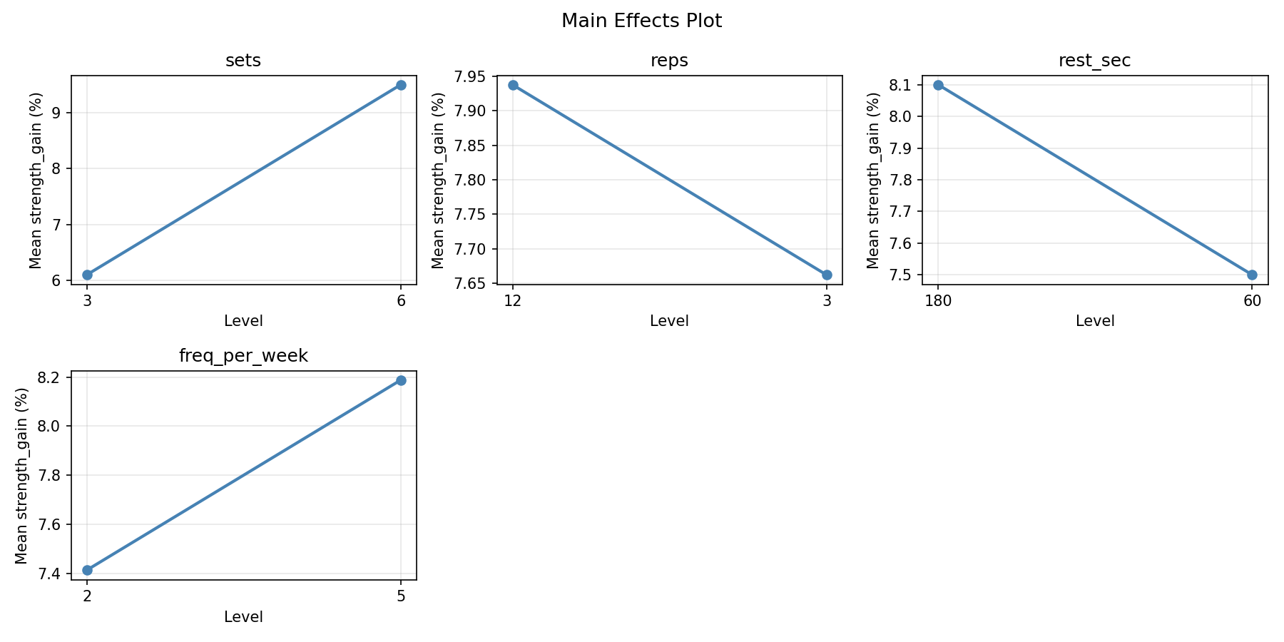
Main Effects Plot
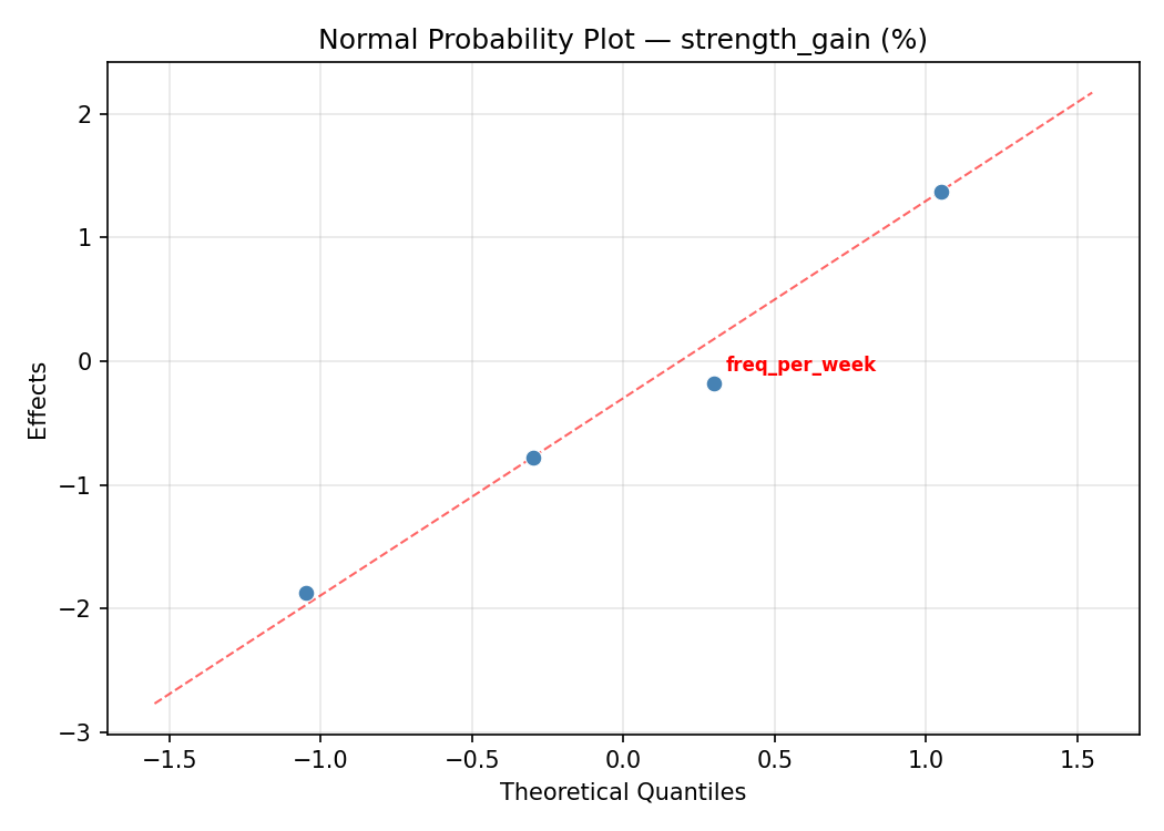
Normal Probability Plot of Effects
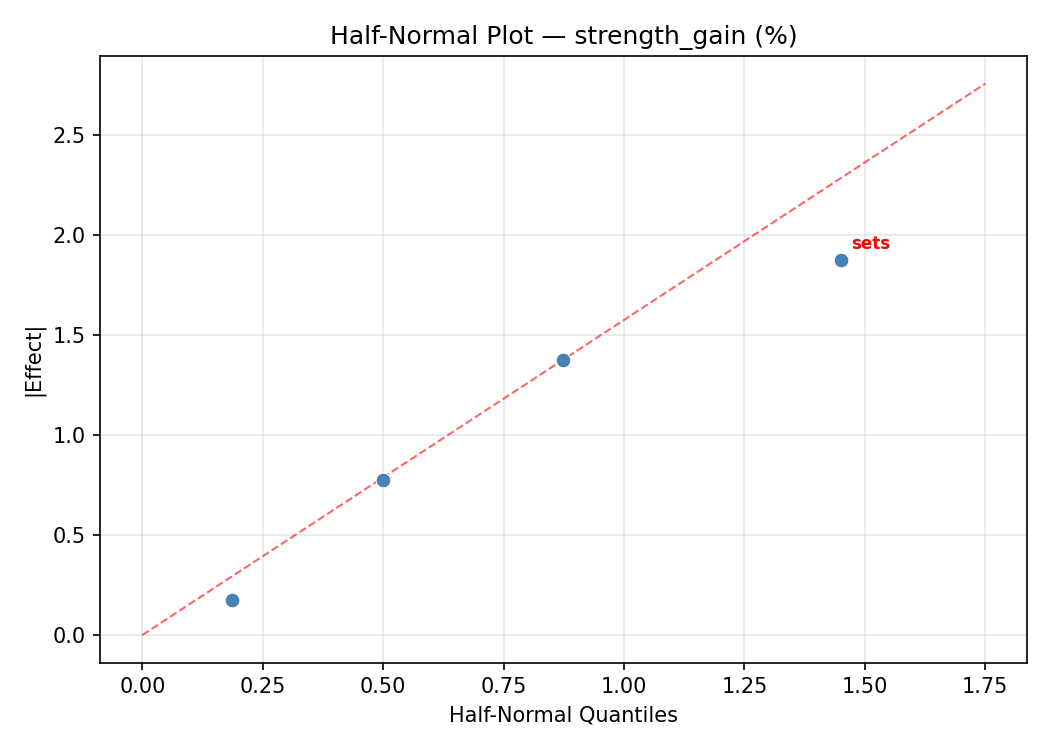
Half-Normal Plot of Effects
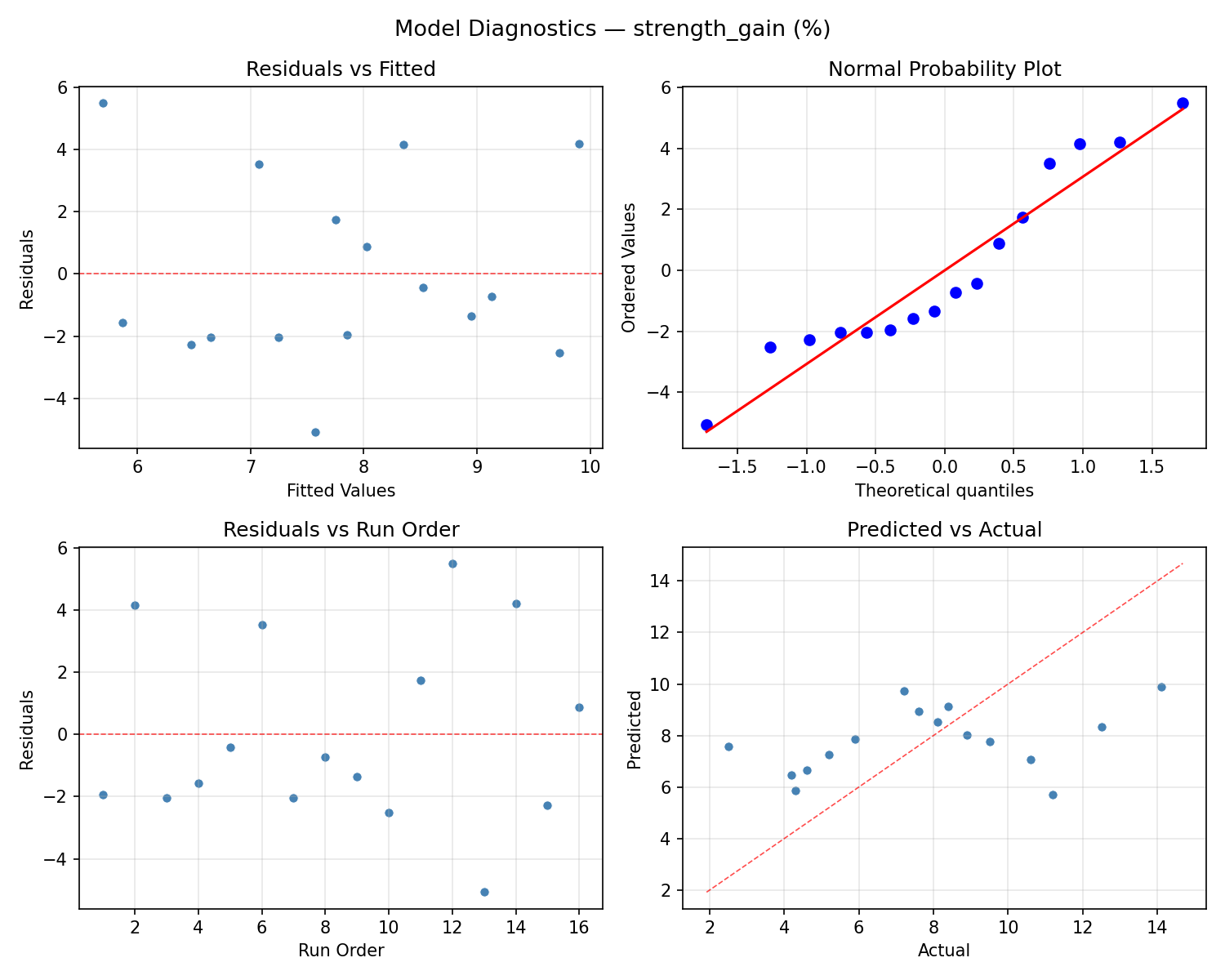
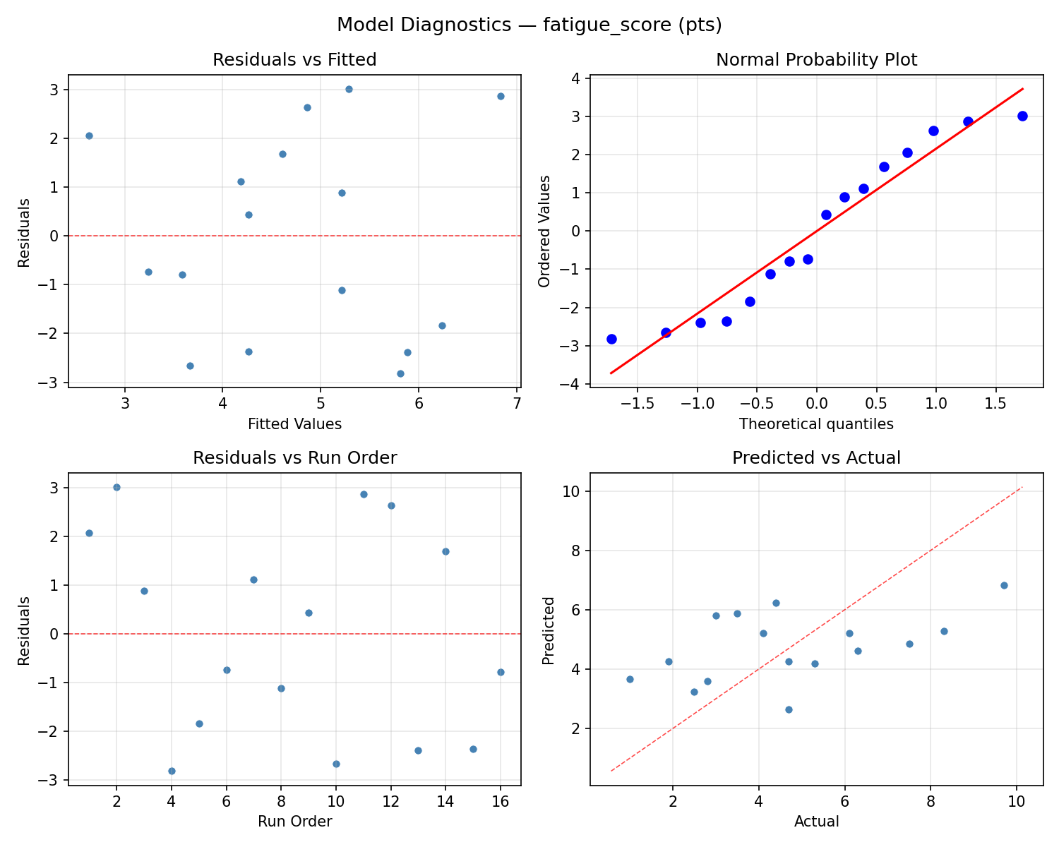
Model Diagnostics
Response: fatigue_score
Top factors: sets (70.8%), reps (19.0%), freq_per_week (6.7%).
ANOVA
| Source | DF | SS | MS | F | p-value |
|---|
| Source | DF | SS | MS | F | p-value |
| sets | 1 | 47.6100 | 47.6100 | 9.525 | 0.0273 |
| reps | 1 | 3.4225 | 3.4225 | 0.685 | 0.4457 |
| rest_sec | 1 | 0.1225 | 0.1225 | 0.025 | 0.8817 |
| freq_per_week | 1 | 0.4225 | 0.4225 | 0.085 | 0.7829 |
| sets*reps | 1 | 3.6100 | 3.6100 | 0.722 | 0.4342 |
| sets*rest_sec | 1 | 0.4900 | 0.4900 | 0.098 | 0.7668 |
| sets*freq_per_week | 1 | 4.0000 | 4.0000 | 0.800 | 0.4120 |
| reps*rest_sec | 1 | 0.3025 | 0.3025 | 0.061 | 0.8155 |
| reps*freq_per_week | 1 | 0.4225 | 0.4225 | 0.085 | 0.7829 |
| rest_sec*freq_per_week | 1 | 0.0225 | 0.0225 | 0.005 | 0.9491 |
| Error | 5 | 24.9925 | 4.9985 | | |
| Total | 15 | 85.4175 | 5.6945 | | |
Pareto Chart
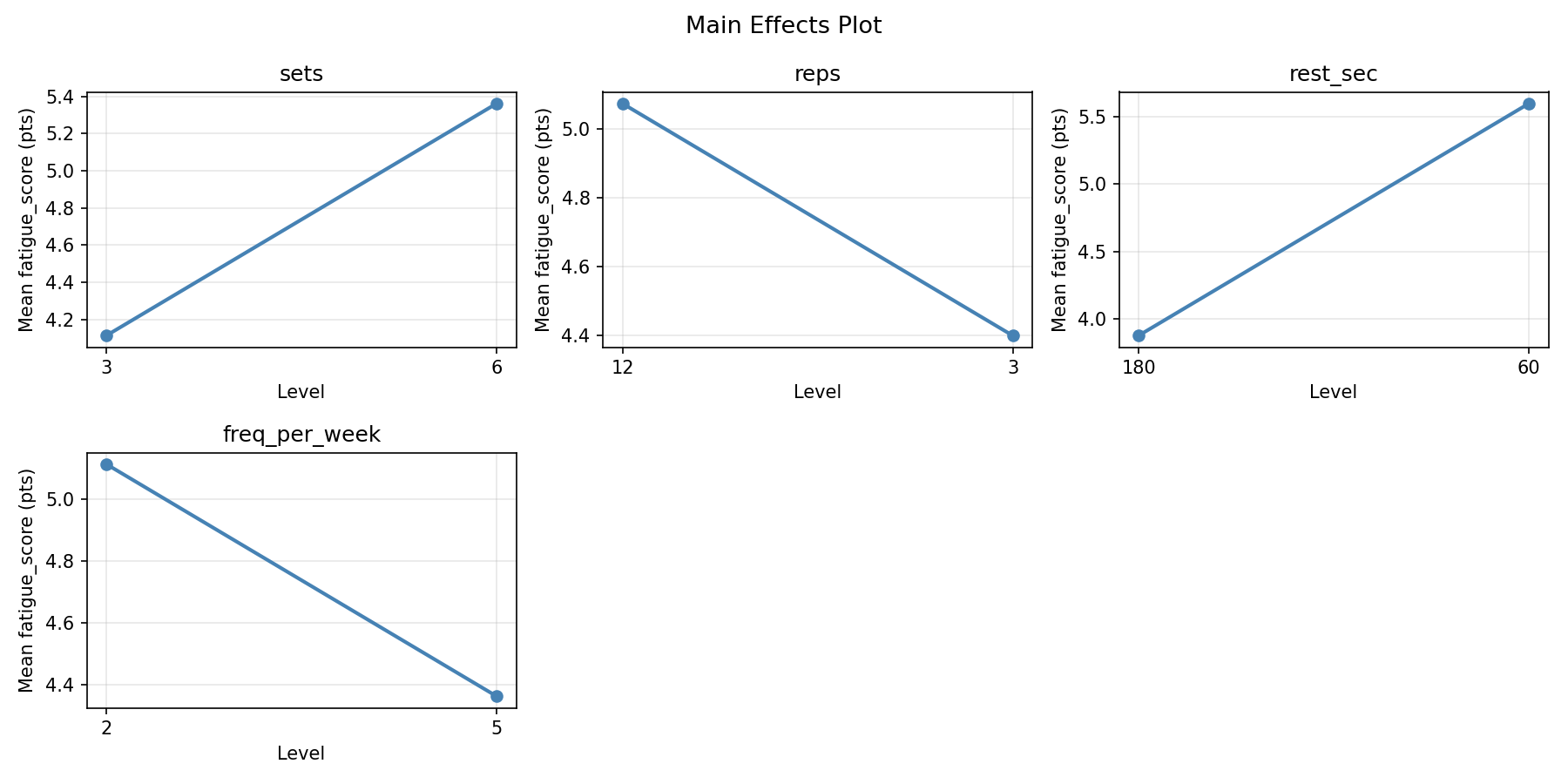
Main Effects Plot
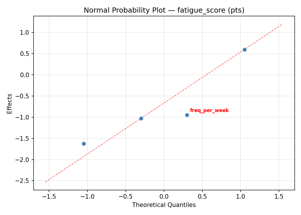
Normal Probability Plot of Effects
Half-Normal Plot of Effects
Model Diagnostics
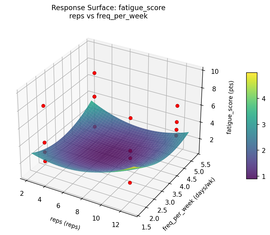
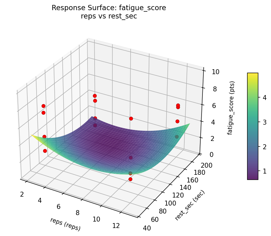
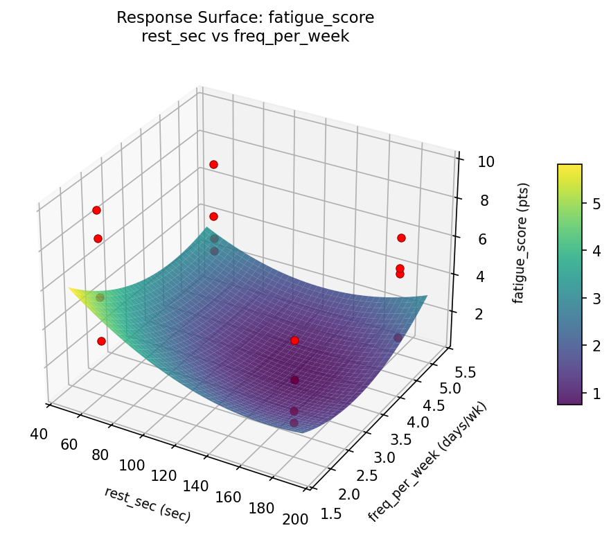
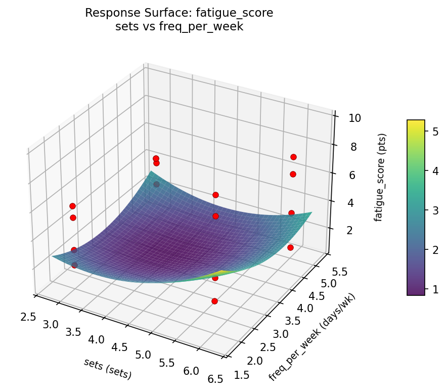
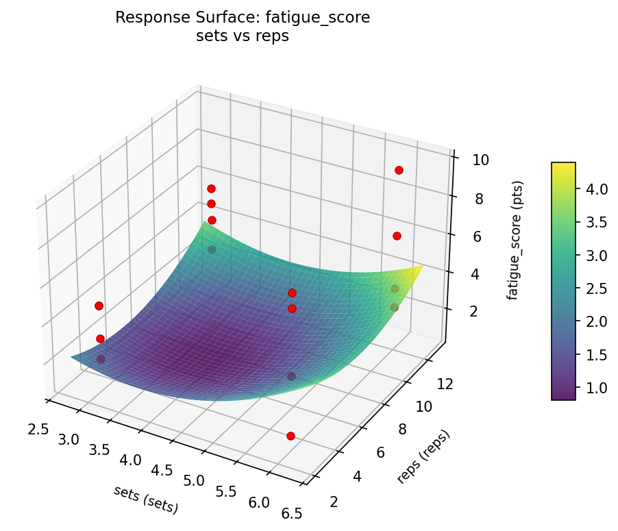
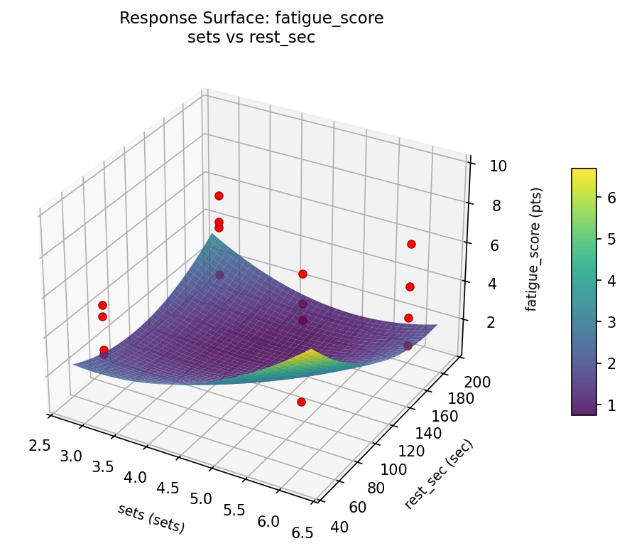
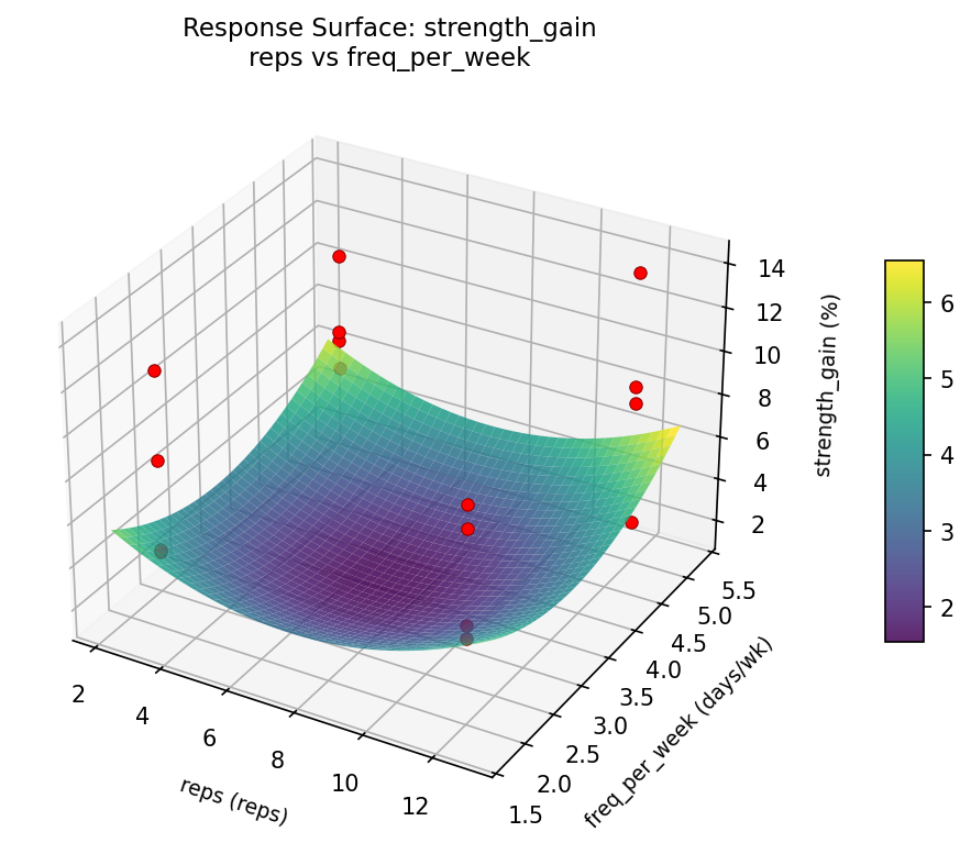
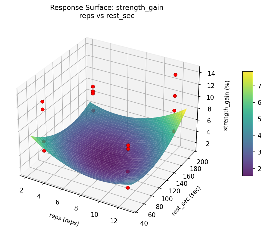
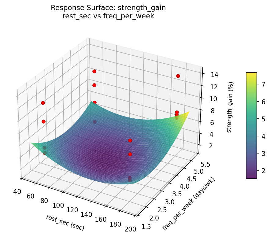
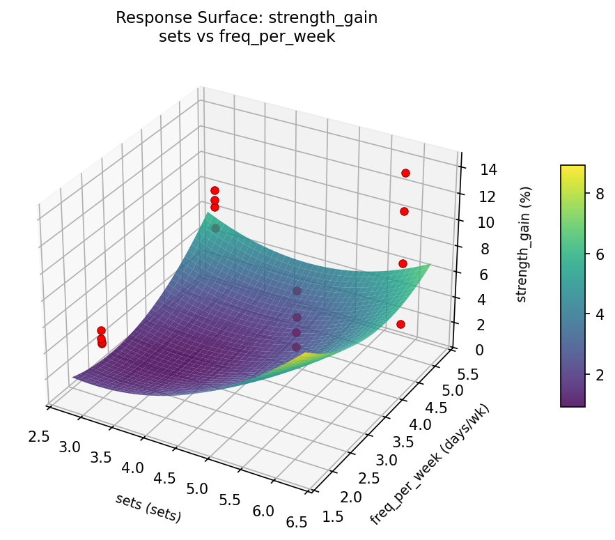
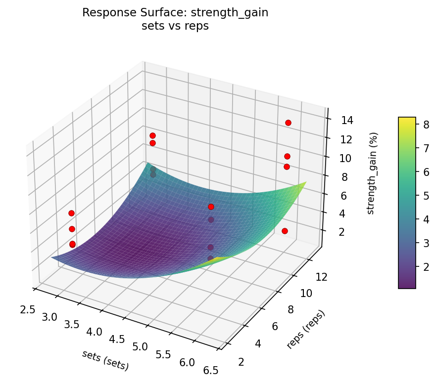
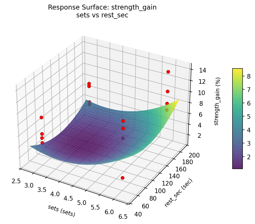
Response Surface Plots
3D surfaces fitted with quadratic RSM. Red dots are observed data points.
fatigue score reps vs freq per week
fatigue score reps vs rest sec
fatigue score rest sec vs freq per week
fatigue score sets vs freq per week
fatigue score sets vs reps
fatigue score sets vs rest sec
strength gain reps vs freq per week
strength gain reps vs rest sec
strength gain rest sec vs freq per week
strength gain sets vs freq per week
strength gain sets vs reps
strength gain sets vs rest sec
Multi-Objective Optimization
When responses compete, Derringer–Suich desirability finds the best compromise.
Each response is scaled to a 0–1 desirability, then combined via a weighted geometric mean.
Overall Desirability
D = 0.7250
Per-Response Desirability
| Response | Weight | Desirability | Predicted | Dir |
|---|
strength_gain |
1.5 |
|
10.60 0.6803 10.60 % |
↑ |
fatigue_score |
1.0 |
|
2.50 0.7978 2.50 pts |
↓ |
Recommended Settings
| Factor | Value |
|---|
sets | 3 sets |
reps | 3 reps |
rest_sec | 60 sec |
freq_per_week | 5 days/wk |
Source: from observed run #6
Trade-off Summary
Sacrifice = how much worse than single-objective best.
| Response | Predicted | Best Observed | Sacrifice |
|---|
fatigue_score | 2.50 | 1.00 | +1.50 |
Top 3 Runs by Desirability
| Run | D | Factor Settings |
|---|
| #14 | 0.6746 | sets=6, reps=3, rest_sec=180, freq_per_week=2 |
| #16 | 0.6260 | sets=3, reps=12, rest_sec=60, freq_per_week=5 |
Model Quality
| Response | R² | Type |
|---|
fatigue_score | 0.2121 | linear |
Full Multi-Objective Output
============================================================
MULTI-OBJECTIVE OPTIMIZATION
Method: Derringer-Suich Desirability Function
============================================================
Overall desirability: D = 0.7250
Response Weight Desirability Predicted Direction
---------------------------------------------------------------------
strength_gain 1.5 0.6803 10.60 % ↑
fatigue_score 1.0 0.7978 2.50 pts ↓
Recommended settings:
sets = 3 sets
reps = 3 reps
rest_sec = 60 sec
freq_per_week = 5 days/wk
(from observed run #6)
Trade-off summary:
strength_gain: 10.60 (best observed: 14.10, sacrifice: +3.50)
fatigue_score: 2.50 (best observed: 1.00, sacrifice: +1.50)
Model quality:
strength_gain: R² = 0.3361 (linear)
fatigue_score: R² = 0.2121 (linear)
Top 3 observed runs by overall desirability:
1. Run #6 (D=0.7250): sets=3, reps=3, rest_sec=60, freq_per_week=5
2. Run #14 (D=0.6746): sets=6, reps=3, rest_sec=180, freq_per_week=2
3. Run #16 (D=0.6260): sets=3, reps=12, rest_sec=60, freq_per_week=5
Full Analysis Output
=== Main Effects: strength_gain ===
Factor Effect Std Error % Contribution
--------------------------------------------------------------
sets -2.8000 0.8166 76.2%
reps -0.3750 0.8166 10.2%
freq_per_week 0.3750 0.8166 10.2%
rest_sec 0.1250 0.8166 3.4%
=== ANOVA Table: strength_gain ===
Source DF SS MS F p-value
-----------------------------------------------------------------------------
sets 1 31.3600 31.3600 1.928 0.2236
reps 1 0.5625 0.5625 0.035 0.8598
rest_sec 1 0.0625 0.0625 0.004 0.9530
freq_per_week 1 0.5625 0.5625 0.035 0.8598
sets*reps 1 3.4225 3.4225 0.210 0.6657
sets*rest_sec 1 6.5025 6.5025 0.400 0.5550
sets*freq_per_week 1 1.8225 1.8225 0.112 0.7514
reps*rest_sec 1 1.6900 1.6900 0.104 0.7602
reps*freq_per_week 1 32.4900 32.4900 1.998 0.2167
rest_sec*freq_per_week 1 0.2500 0.2500 0.015 0.9062
Error 5 81.3150 16.2630
Total 15 160.0400 10.6693
=== Interaction Effects: strength_gain ===
Factor A Factor B Interaction % Contribution
------------------------------------------------------------------------
reps freq_per_week -2.8500 43.0%
sets rest_sec -1.2750 19.2%
sets reps 0.9250 14.0%
sets freq_per_week -0.6750 10.2%
reps rest_sec -0.6500 9.8%
rest_sec freq_per_week 0.2500 3.8%
=== Summary Statistics: strength_gain ===
sets:
Level N Mean Std Min Max
------------------------------------------------------------
3 8 9.2000 3.3381 4.6000 14.1000
6 8 6.4000 2.6907 2.5000 10.6000
reps:
Level N Mean Std Min Max
------------------------------------------------------------
12 8 7.9875 3.7296 2.5000 14.1000
3 8 7.6125 2.9787 4.2000 12.5000
rest_sec:
Level N Mean Std Min Max
------------------------------------------------------------
180 8 7.7375 2.8685 2.5000 11.2000
60 8 7.8625 3.8243 4.2000 14.1000
freq_per_week:
Level N Mean Std Min Max
------------------------------------------------------------
2 8 7.6125 3.4873 2.5000 12.5000
5 8 7.9875 3.2590 4.3000 14.1000
=== Main Effects: fatigue_score ===
Factor Effect Std Error % Contribution
--------------------------------------------------------------
sets -3.4500 0.5966 70.8%
reps -0.9250 0.5966 19.0%
freq_per_week -0.3250 0.5966 6.7%
rest_sec -0.1750 0.5966 3.6%
=== ANOVA Table: fatigue_score ===
Source DF SS MS F p-value
-----------------------------------------------------------------------------
sets 1 47.6100 47.6100 9.525 0.0273
reps 1 3.4225 3.4225 0.685 0.4457
rest_sec 1 0.1225 0.1225 0.025 0.8817
freq_per_week 1 0.4225 0.4225 0.085 0.7829
sets*reps 1 3.6100 3.6100 0.722 0.4342
sets*rest_sec 1 0.4900 0.4900 0.098 0.7668
sets*freq_per_week 1 4.0000 4.0000 0.800 0.4120
reps*rest_sec 1 0.3025 0.3025 0.061 0.8155
reps*freq_per_week 1 0.4225 0.4225 0.085 0.7829
rest_sec*freq_per_week 1 0.0225 0.0225 0.005 0.9491
Error 5 24.9925 4.9985
Total 15 85.4175 5.6945
=== Interaction Effects: fatigue_score ===
Factor A Factor B Interaction % Contribution
------------------------------------------------------------------------
sets freq_per_week 1.0000 33.6%
sets reps 0.9500 31.9%
sets rest_sec 0.3500 11.8%
reps freq_per_week 0.3250 10.9%
reps rest_sec 0.2750 9.2%
rest_sec freq_per_week 0.0750 2.5%
=== Summary Statistics: fatigue_score ===
sets:
Level N Mean Std Min Max
------------------------------------------------------------
3 8 6.4625 1.9376 4.1000 9.7000
6 8 3.0125 1.2833 1.0000 4.7000
reps:
Level N Mean Std Min Max
------------------------------------------------------------
12 8 5.2000 2.7800 1.0000 9.7000
3 8 4.2750 1.9962 1.9000 8.3000
rest_sec:
Level N Mean Std Min Max
------------------------------------------------------------
180 8 4.8250 2.7551 1.0000 9.7000
60 8 4.6500 2.1434 1.9000 8.3000
freq_per_week:
Level N Mean Std Min Max
------------------------------------------------------------
2 8 4.9000 2.8641 1.9000 9.7000
5 8 4.5750 1.9848 1.0000 7.5000
Optimization Recommendations
=== Optimization: strength_gain ===
Direction: maximize
Best observed run: #14
sets = 6
reps = 12
rest_sec = 60
freq_per_week = 2
Value: 14.1
RSM Model (linear, R² = 0.2001, Adj R² = -0.0908):
Coefficients:
intercept +7.8000
sets -0.2750
reps -0.9125
rest_sec -0.7875
freq_per_week -0.6875
RSM Model (quadratic, R² = 0.4241, Adj R² = -7.6392):
Coefficients:
intercept +1.5600
sets -0.2750
reps -0.9125
rest_sec -0.7875
freq_per_week -0.6875
sets*reps -0.2375
sets*rest_sec -0.6625
sets*freq_per_week -0.7375
reps*rest_sec +0.6750
reps*freq_per_week -0.8000
rest_sec*freq_per_week +0.3250
sets^2 +1.5600
reps^2 +1.5600
rest_sec^2 +1.5600
freq_per_week^2 +1.5600
Curvature analysis:
sets coef=+1.5600 convex (has a minimum)
reps coef=+1.5600 convex (has a minimum)
rest_sec coef=+1.5600 convex (has a minimum)
freq_per_week coef=+1.5600 convex (has a minimum)
Notable interactions:
reps*freq_per_week coef=-0.8000 (antagonistic)
sets*freq_per_week coef=-0.7375 (antagonistic)
reps*rest_sec coef=+0.6750 (synergistic)
sets*rest_sec coef=-0.6625 (antagonistic)
rest_sec*freq_per_week coef=+0.3250 (synergistic)
Predicted optimum (from linear model, at observed points):
sets = 3
reps = 3
rest_sec = 60
freq_per_week = 2
Predicted value: 10.4625
Surface optimum (via L-BFGS-B, linear model):
sets = 3
reps = 3
rest_sec = 60
freq_per_week = 2
Predicted value: 10.4625
Model quality: Weak fit — consider adding center points or using a different design.
Factor importance:
1. reps (effect: 1.8, contribution: 34.3%)
2. rest_sec (effect: 1.6, contribution: 29.6%)
3. freq_per_week (effect: -1.4, contribution: 25.8%)
4. sets (effect: -0.5, contribution: 10.3%)
=== Optimization: fatigue_score ===
Direction: minimize
Best observed run: #10
sets = 3
reps = 12
rest_sec = 60
freq_per_week = 5
Value: 1.0
RSM Model (linear, R² = 0.4137, Adj R² = 0.2005):
Coefficients:
intercept +4.7375
sets +0.9125
reps -1.1125
rest_sec +0.2750
freq_per_week +0.2500
RSM Model (quadratic, R² = 0.6912, Adj R² = -3.6321):
Coefficients:
intercept +0.9475
sets +0.9125
reps -1.1125
rest_sec +0.2750
freq_per_week +0.2500
sets*reps +0.1875
sets*rest_sec -0.0500
sets*freq_per_week -0.7500
reps*rest_sec +0.1750
reps*freq_per_week -0.8250
rest_sec*freq_per_week +0.4125
sets^2 +0.9475
reps^2 +0.9475
rest_sec^2 +0.9475
freq_per_week^2 +0.9475
Curvature analysis:
freq_per_week coef=+0.9475 convex (has a minimum)
sets coef=+0.9475 convex (has a minimum)
reps coef=+0.9475 convex (has a minimum)
rest_sec coef=+0.9475 convex (has a minimum)
Notable interactions:
reps*freq_per_week coef=-0.8250 (antagonistic)
sets*freq_per_week coef=-0.7500 (antagonistic)
rest_sec*freq_per_week coef=+0.4125 (synergistic)
Predicted optimum (from linear model, at observed points):
sets = 6
reps = 3
rest_sec = 180
freq_per_week = 5
Predicted value: 7.2875
Surface optimum (via L-BFGS-B, linear model):
sets = 3
reps = 12
rest_sec = 60
freq_per_week = 2
Predicted value: 2.1875
Model quality: Weak fit — consider adding center points or using a different design.
Factor importance:
1. reps (effect: 2.2, contribution: 43.6%)
2. sets (effect: 1.8, contribution: 35.8%)
3. rest_sec (effect: -0.5, contribution: 10.8%)
4. freq_per_week (effect: 0.5, contribution: 9.8%)