Summary
This experiment investigates infiniband network tuning. Box-Behnken design to optimize InfiniBand HDR network throughput and tail latency.
The design varies 3 factors: mtu (bytes), ranging from 2048 to 4096, queue depth, ranging from 64 to 512, and rdma cm, ranging from 0 to 1. The goal is to optimize 2 responses: msg rate (Mmsg/s) (maximize) and p99 lat (us) (minimize). Fixed conditions held constant across all runs include ib speed = HDR, ports = 1.
A Box-Behnken design was chosen because it efficiently fits quadratic models with 3 continuous factors while avoiding extreme corner combinations — requiring only 15 runs instead of the 8 needed for a full factorial at two levels.
Quadratic response surface models were fitted to capture potential curvature and factor interactions. The RSM contour plots below visualize how pairs of factors jointly affect each response.
Key Findings
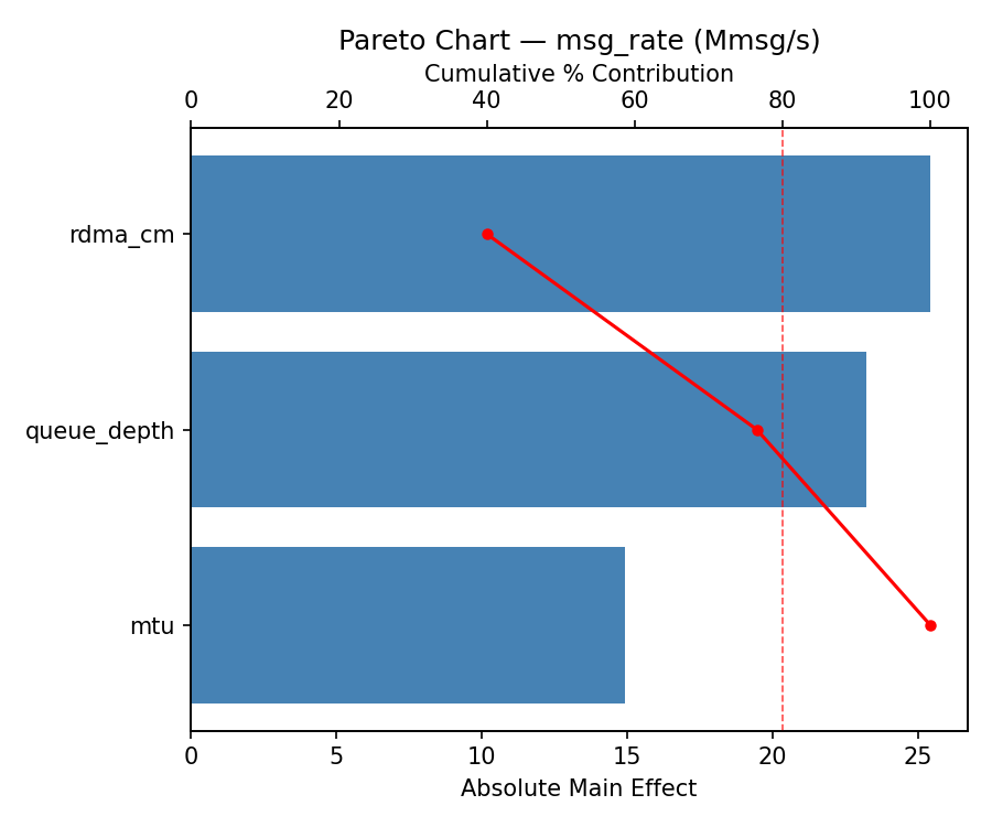
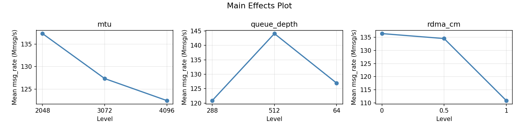
For msg rate, the most influential factors were mtu (38.2%), queue depth (34.7%), rdma cm (27.1%). The best observed value was 161.8 (at mtu = 3072, queue depth = 288, rdma cm = 0.5).
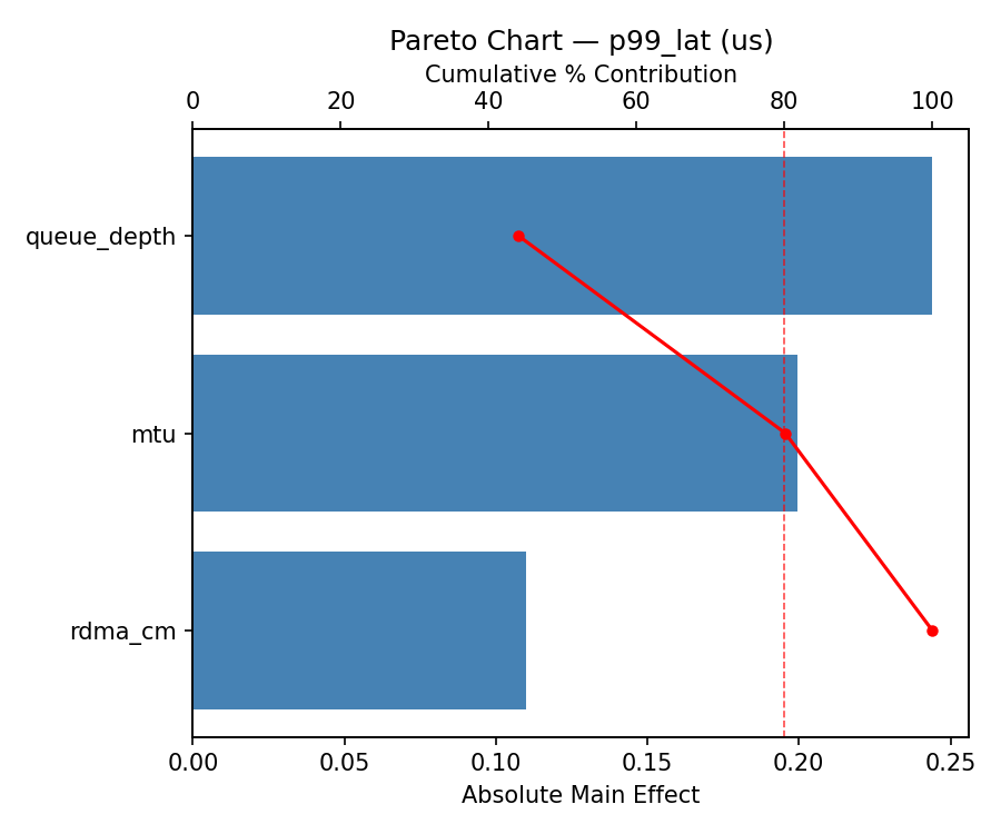
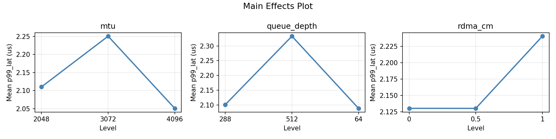
For p99 lat, the most influential factors were rdma cm (34.8%), mtu (34.5%), queue depth (30.6%). The best observed value was 1.854 (at mtu = 4096, queue depth = 288, rdma cm = 0).
Recommended Next Steps
- Run confirmation experiments at the predicted optimal settings to validate the model.
- Consider whether any fixed factors should be varied in a future study.
Experimental Setup
Factors
| Factor | Levels | Type | Unit |
|---|---|---|---|
mtu | 2048, 4096 | continuous | bytes |
queue_depth | 64, 512 | continuous | |
rdma_cm | 0, 1 | continuous |
Fixed: ib_speed=HDR, ports=1
Responses
| Response | Direction | Unit |
|---|---|---|
msg_rate | ↑ maximize | Mmsg/s |
p99_lat | ↓ minimize | us |
Experimental Matrix
The Box-Behnken Design produces 15 runs. Each row is one experiment with specific factor settings.
| Run | mtu | queue_depth | rdma_cm |
|---|---|---|---|
| 1 | 3072 | 64 | 0 |
| 2 | 3072 | 288 | 0.5 |
| 3 | 4096 | 288 | 1 |
| 4 | 4096 | 288 | 0 |
| 5 | 3072 | 288 | 0.5 |
| 6 | 3072 | 288 | 0.5 |
| 7 | 2048 | 288 | 1 |
| 8 | 4096 | 64 | 0.5 |
| 9 | 3072 | 64 | 1 |
| 10 | 4096 | 512 | 0.5 |
| 11 | 2048 | 288 | 0 |
| 12 | 3072 | 512 | 1 |
| 13 | 2048 | 64 | 0.5 |
| 14 | 2048 | 512 | 0.5 |
| 15 | 3072 | 512 | 0 |
How to Run
Analysis Results
Generated from actual experiment runs.
Response: msg_rate
Pareto Chart
Main Effects Plot
Response: p99_lat
Pareto Chart
Main Effects Plot
Response Surface Plots
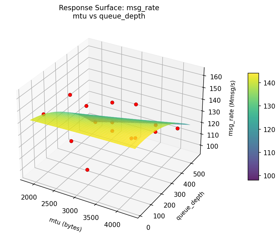
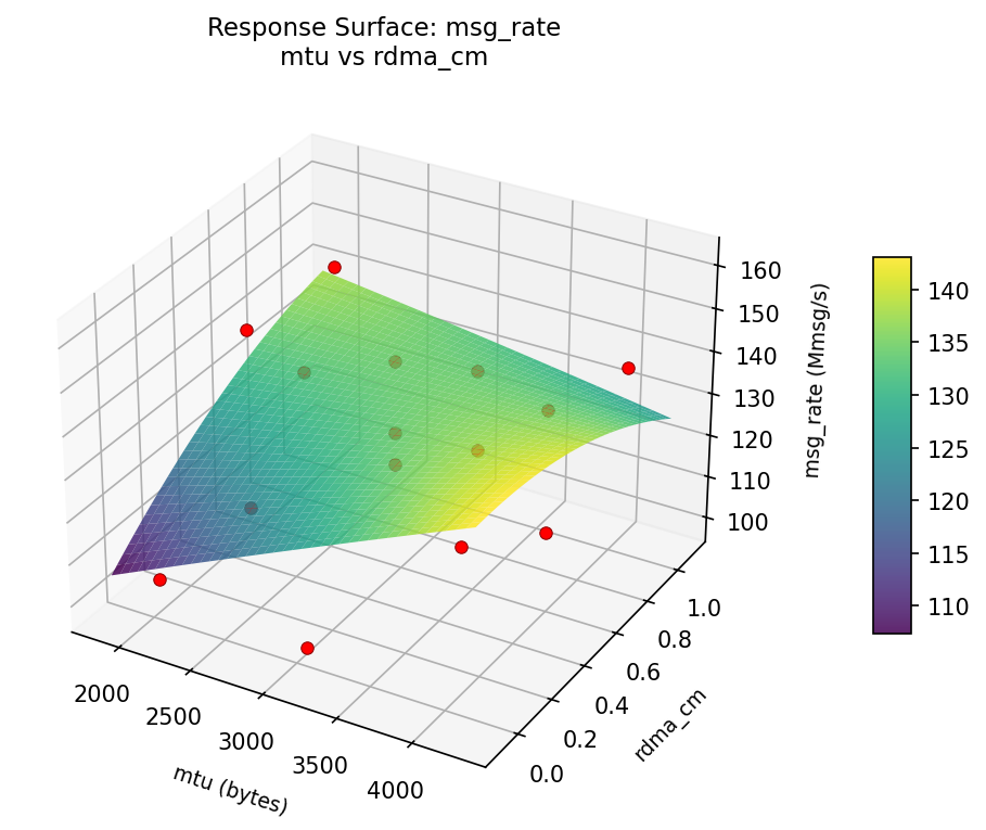
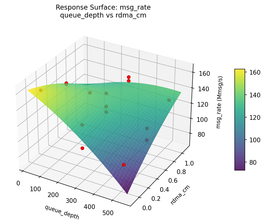
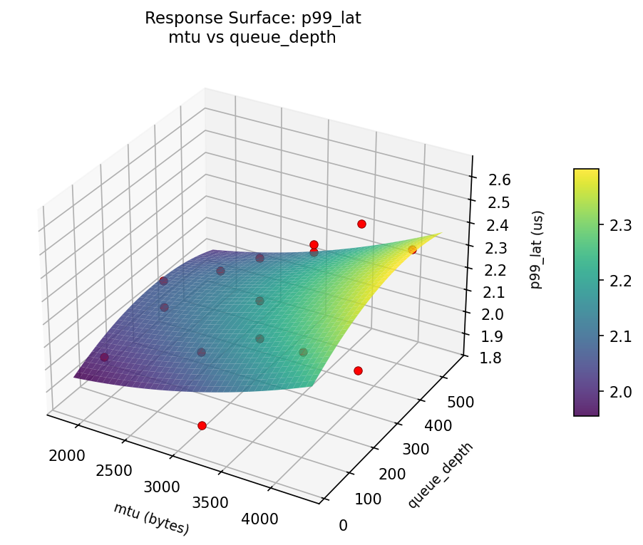
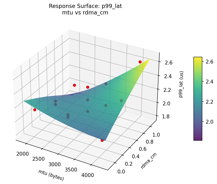
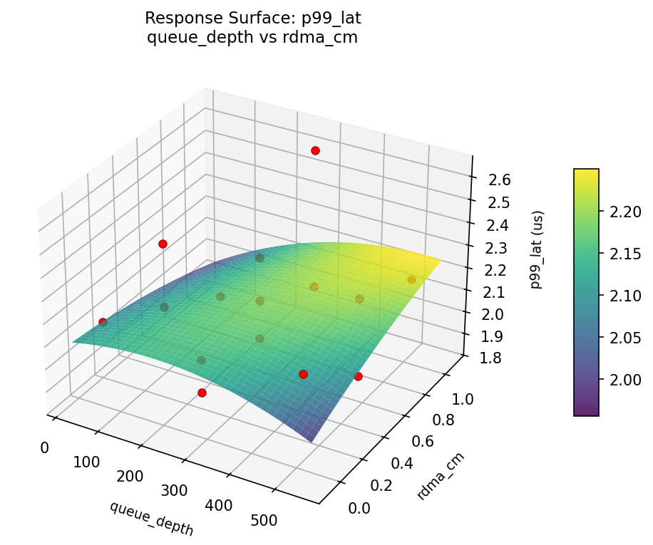
3D surfaces fitted with quadratic RSM. Red dots are observed data points.
How to Read These Surfaces
Each plot shows predicted response (vertical axis) across two factors while other factors are held at center. Red dots are actual experimental observations.
- Flat surface — these two factors have little effect on the response.
- Tilted plane — strong linear effect; moving along one axis consistently changes the response.
- Curved/domed surface — quadratic curvature; there is an optimum somewhere in the middle.
- Saddle shape — significant interaction; the best setting of one factor depends on the other.
- Red dots far from surface — poor model fit in that region; be cautious about predictions there.
msg_rate (Mmsg/s) — R² = 0.864, Adj R² = 0.618
The model fits well — the surface shape is reliable.
Curvature detected in mtu, rdma_cm — look for a peak or valley in the surface.
Strongest linear driver: rdma_cm (increases msg_rate).
Notable interaction: mtu × rdma_cm — the effect of one depends on the level of the other. Look for a twisted surface.
p99_lat (us) — R² = 0.622, Adj R² = -0.058
Moderate fit — surface shows general trends but some noise remains.
Strongest linear driver: queue_depth (increases p99_lat).
msg: rate mtu vs queue depth
msg: rate mtu vs rdma cm
msg: rate queue depth vs rdma cm
p99: lat mtu vs queue depth
p99: lat mtu vs rdma cm
p99: lat queue depth vs rdma cm
Full Analysis Output
Optimization Recommendations
Multi-Objective Optimization
When responses compete, Derringer–Suich desirability finds the best compromise. Each response is scaled to a 0–1 desirability, then combined via a weighted geometric mean.
Per-Response Desirability
| Response | Weight | Desirability | Predicted | Dir |
|---|---|---|---|---|
msg_rate |
1.5 |
0.9545
|
161.80 0.9545 161.80 Mmsg/s | ↑ |
p99_lat |
1.0 |
0.5760
|
2.18 0.5760 2.18 us | ↓ |
Recommended Settings
| Factor | Value |
|---|---|
mtu | 3072 bytes |
queue_depth | 288 |
rdma_cm | 0.5 |
Source: from observed run #10
Trade-off Summary
Sacrifice = how much worse than single-objective best.
| Response | Predicted | Best Observed | Sacrifice |
|---|---|---|---|
p99_lat | 2.18 | 1.85 | +0.32 |
Top 3 Runs by Desirability
| Run | D | Factor Settings |
|---|---|---|
| #4 | 0.7311 | mtu=2048, queue_depth=288, rdma_cm=1 |
| #3 | 0.7200 | mtu=3072, queue_depth=512, rdma_cm=1 |
Model Quality
| Response | R² | Type |
|---|---|---|
p99_lat | 0.8835 | quadratic |