Summary
This experiment investigates job scheduler packing optimization. Optimize HPC job scheduler packing parameters to maximize throughput and resource efficiency.
The design varies 3 factors: nodes (count), ranging from 4 to 64, tasks per node (count), ranging from 8 to 48, and mem per task (GB), ranging from 1 to 8. The goal is to optimize 2 responses: throughput (jobs/h) (maximize) and efficiency (%) (maximize).
A Central Composite Design (CCD) was selected to fit a full quadratic response surface model, including curvature and interaction effects. With 3 factors this produces 22 runs including center points and axial (star) points that extend beyond the factorial range.
Quadratic response surface models were fitted to capture potential curvature and factor interactions. The RSM contour plots below visualize how pairs of factors jointly affect each response.
Key Findings
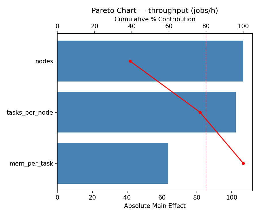
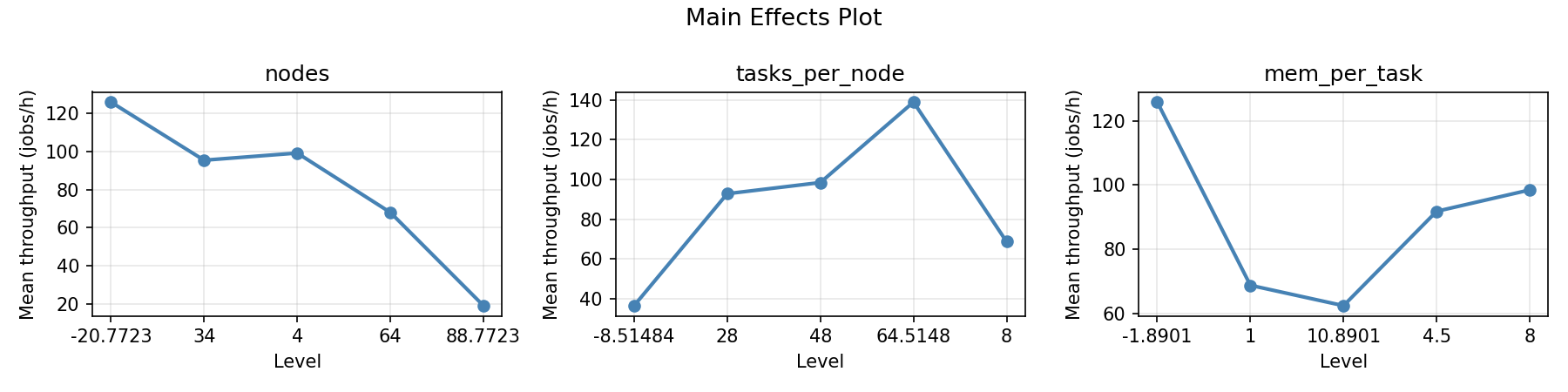
For throughput, the most influential factors were tasks per node (34.4%), mem per task (34.0%), nodes (31.7%). The best observed value was 261.62 (at nodes = 64, tasks per node = 48, mem per task = 1).
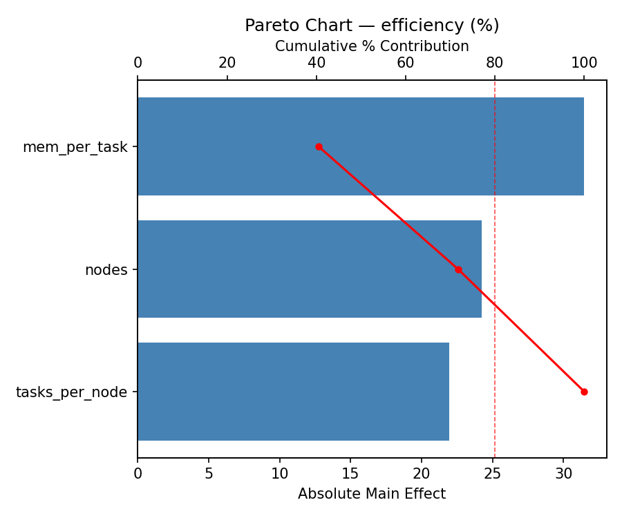
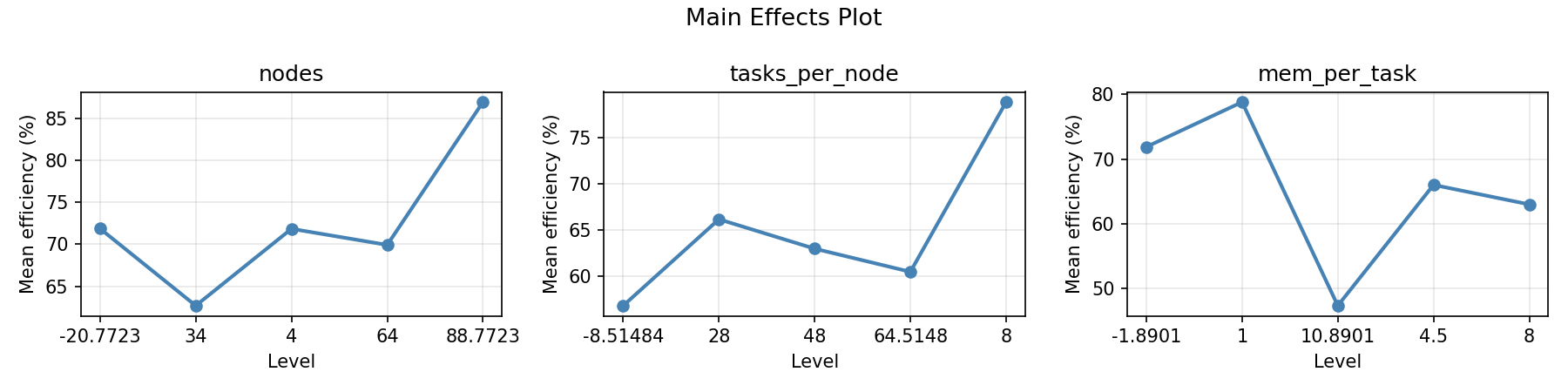
For efficiency, the most influential factors were tasks per node (40.1%), nodes (37.1%), mem per task (22.8%). The best observed value was 86.93 (at nodes = 34, tasks per node = 28, mem per task = 4.5).
Recommended Next Steps
- Run confirmation experiments at the predicted optimal settings to validate the model.
- Consider whether any fixed factors should be varied in a future study.
Experimental Setup
Factors
| Factor | Levels | Type | Unit |
|---|---|---|---|
nodes | 4, 64 | continuous | count |
tasks_per_node | 8, 48 | continuous | count |
mem_per_task | 1, 8 | continuous | GB |
Fixed: none
Responses
| Response | Direction | Unit |
|---|---|---|
throughput | ↑ maximize | jobs/h |
efficiency | ↑ maximize | % |
Experimental Matrix
The Central Composite Design produces 22 runs. Each row is one experiment with specific factor settings.
| Run | nodes | tasks_per_node | mem_per_task |
|---|---|---|---|
| 1 | 34 | 28 | 4.5 |
| 2 | 64 | 8 | 8 |
| 3 | 4 | 48 | 1 |
| 4 | 34 | 64.5148 | 4.5 |
| 5 | 34 | 28 | 4.5 |
| 6 | -20.7723 | 28 | 4.5 |
| 7 | 34 | 28 | -1.8901 |
| 8 | 34 | 28 | 4.5 |
| 9 | 64 | 48 | 1 |
| 10 | 88.7723 | 28 | 4.5 |
| 11 | 34 | 28 | 4.5 |
| 12 | 34 | -8.51484 | 4.5 |
| 13 | 34 | 28 | 4.5 |
| 14 | 4 | 8 | 8 |
| 15 | 34 | 28 | 4.5 |
| 16 | 64 | 8 | 1 |
| 17 | 34 | 28 | 10.8901 |
| 18 | 64 | 48 | 8 |
| 19 | 34 | 28 | 4.5 |
| 20 | 4 | 8 | 1 |
| 21 | 4 | 48 | 8 |
| 22 | 34 | 28 | 4.5 |
How to Run
Analysis Results
Generated from actual experiment runs.
Response: throughput
Pareto Chart
Main Effects Plot
Response: efficiency
Pareto Chart
Main Effects Plot
Response Surface Plots
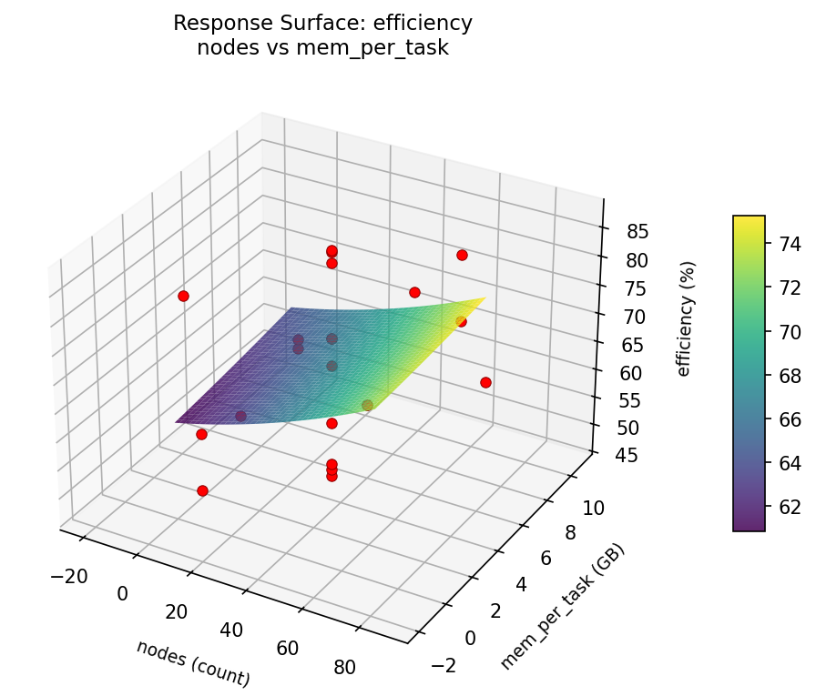
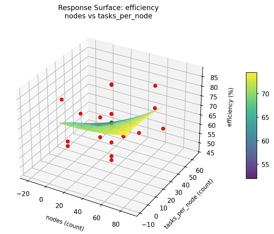
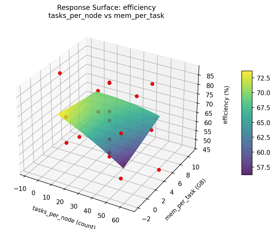
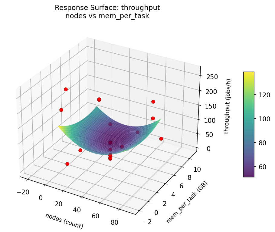
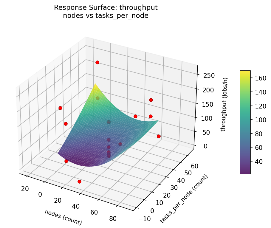
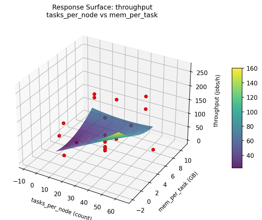
3D surfaces fitted with quadratic RSM. Red dots are observed data points.
How to Read These Surfaces
Each plot shows predicted response (vertical axis) across two factors while other factors are held at center. Red dots are actual experimental observations.
- Flat surface — these two factors have little effect on the response.
- Tilted plane — strong linear effect; moving along one axis consistently changes the response.
- Curved/domed surface — quadratic curvature; there is an optimum somewhere in the middle.
- Saddle shape — significant interaction; the best setting of one factor depends on the other.
- Red dots far from surface — poor model fit in that region; be cautious about predictions there.
throughput (jobs/h) — R² = 0.653, Adj R² = 0.393
Moderate fit — surface shows general trends but some noise remains.
Curvature detected in tasks_per_node, nodes — look for a peak or valley in the surface.
Strongest linear driver: nodes (decreases throughput).
Notable interaction: nodes × tasks_per_node — the effect of one depends on the level of the other. Look for a twisted surface.
efficiency (%) — R² = 0.785, Adj R² = 0.624
Moderate fit — surface shows general trends but some noise remains.
Curvature detected in tasks_per_node, mem_per_task — look for a peak or valley in the surface.
Strongest linear driver: nodes (increases efficiency).
Notable interaction: nodes × tasks_per_node — the effect of one depends on the level of the other. Look for a twisted surface.
efficiency: nodes vs mem per task
efficiency: nodes vs tasks per node
efficiency: tasks per node vs mem per task
throughput: nodes vs mem per task
throughput: nodes vs tasks per node
throughput: tasks per node vs mem per task
Full Analysis Output
Optimization Recommendations
Multi-Objective Optimization
When responses compete, Derringer–Suich desirability finds the best compromise. Each response is scaled to a 0–1 desirability, then combined via a weighted geometric mean.
Per-Response Desirability
| Response | Weight | Desirability | Predicted | Dir |
|---|---|---|---|---|
throughput |
1.5 |
0.6733
|
182.22 0.6733 182.22 jobs/h | ↑ |
efficiency |
1.0 |
0.8723
|
83.35 0.8723 83.35 % | ↑ |
Recommended Settings
| Factor | Value |
|---|---|
nodes | 4 count |
tasks_per_node | 48 count |
mem_per_task | 8 GB |
Source: from observed run #7
Trade-off Summary
Sacrifice = how much worse than single-objective best.
| Response | Predicted | Best Observed | Sacrifice |
|---|---|---|---|
efficiency | 83.35 | 86.93 | +3.58 |
Top 3 Runs by Desirability
| Run | D | Factor Settings |
|---|---|---|
| #1 | 0.5235 | nodes=64, tasks_per_node=8, mem_per_task=8 |
| #5 | 0.5235 | nodes=88.7723, tasks_per_node=28, mem_per_task=4.5 |
Model Quality
| Response | R² | Type |
|---|---|---|
efficiency | 0.0177 | linear |