Tire Pressure & Fuel Economy

Summary

This experiment investigates tire pressure & fuel economy. Box-Behnken design to maximize fuel economy and minimize tire wear by tuning front pressure, rear pressure, and load weight.

The design varies 3 factors: front psi (psi), ranging from 28 to 38, rear psi (psi), ranging from 28 to 38, and load kg (kg), ranging from 100 to 400. The goal is to optimize 2 responses: mpg (mpg) (maximize) and wear rate (mm/10k_mi) (minimize). Fixed conditions held constant across all runs include vehicle = sedan, tire model = all_season.

A Box-Behnken design was chosen because it efficiently fits quadratic models with 3 continuous factors while avoiding extreme corner combinations — requiring only 15 runs instead of the 8 needed for a full factorial at two levels.

Quadratic response surface models were fitted to capture potential curvature and factor interactions. The RSM contour plots below visualize how pairs of factors jointly affect each response.

Key Findings

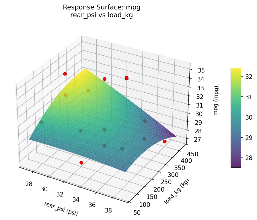
For mpg, the most influential factors were rear psi (47.8%), front psi (38.3%), load kg (13.9%). The best observed value was 35.1 (at front psi = 33, rear psi = 38, load kg = 400).

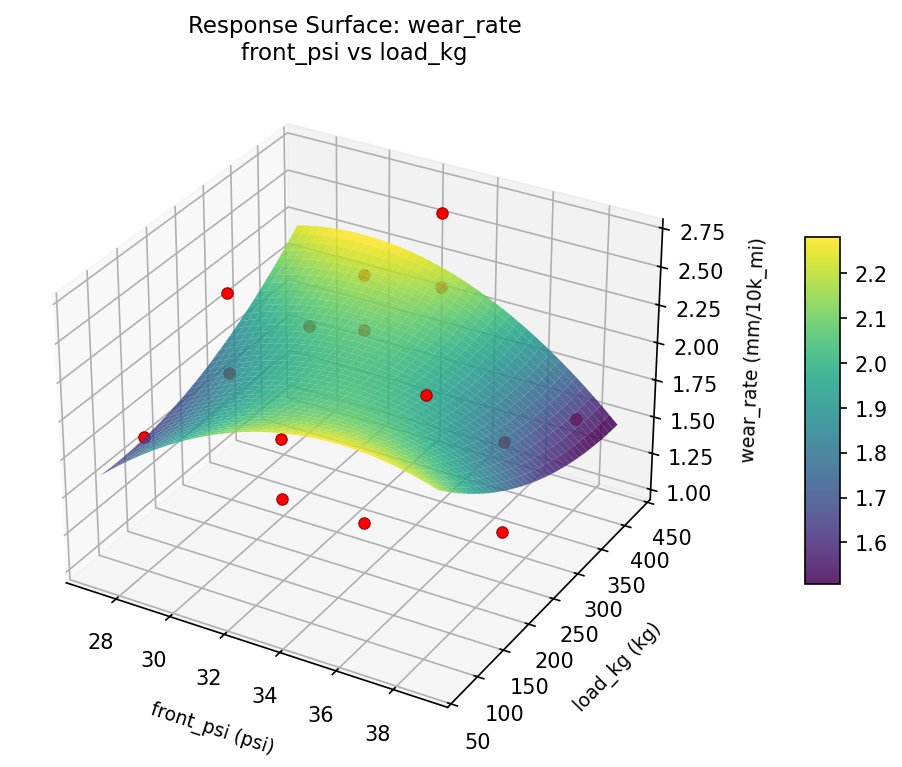
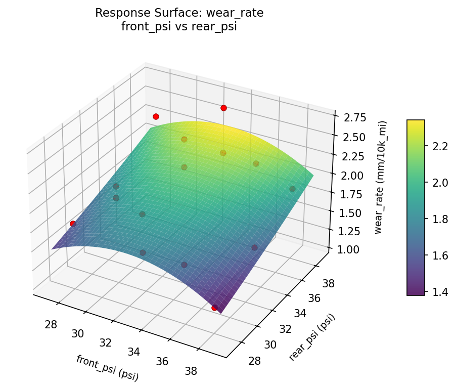
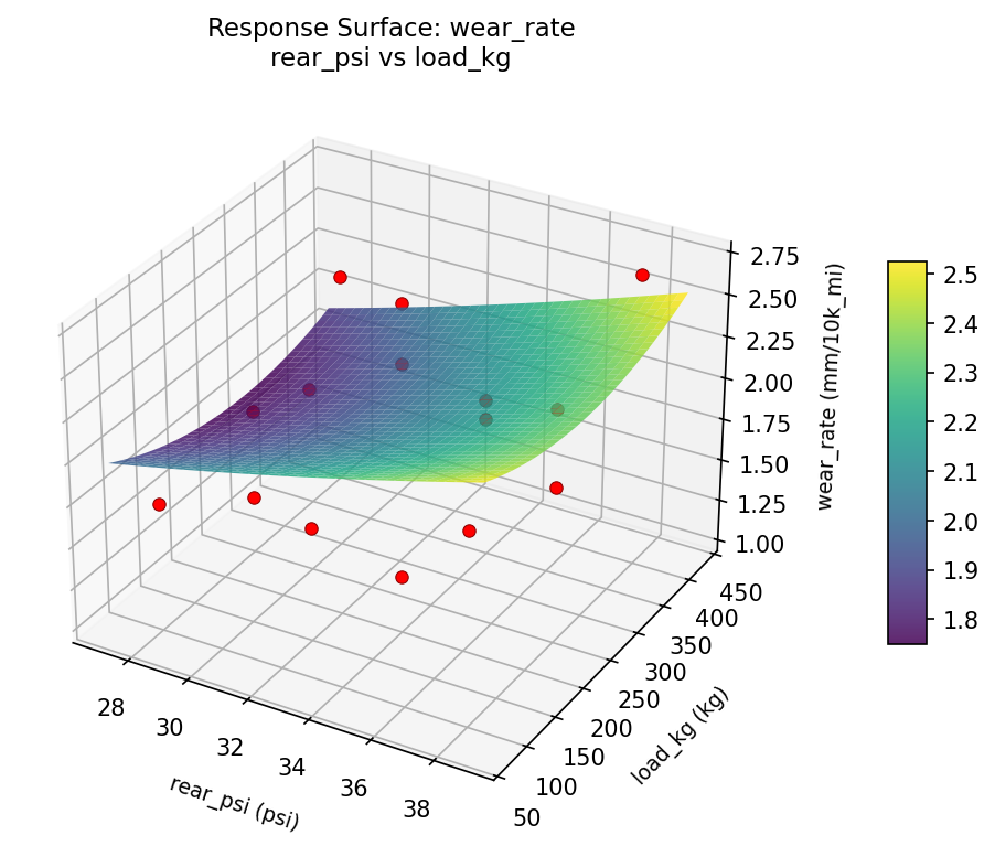
For wear rate, the most influential factors were rear psi (43.6%), front psi (34.4%), load kg (22.0%). The best observed value was 1.05 (at front psi = 33, rear psi = 38, load kg = 400).

Recommended Next Steps

Run confirmation experiments at the predicted optimal settings to validate the model.
Consider whether any fixed factors should be varied in a future study.

Experimental Setup

Factors

Factor	Low	High	Unit
`front_psi`	28	38	psi
`rear_psi`	28	38	psi
`load_kg`	100	400	kg

Fixed: vehicle = sedan, tire_model = all_season

Responses

Response	Direction	Unit
`mpg`	↑ maximize	mpg
`wear_rate`	↓ minimize	mm/10k_mi

Configuration

use_cases/117_tire_pressure_fuel/config.json

{
  "metadata": {
    "name": "Tire Pressure & Fuel Economy",
    "description": "Box-Behnken design to maximize fuel economy and minimize tire wear by tuning front pressure, rear pressure, and load weight"
  },
  "factors": [
    {
      "name": "front_psi",
      "levels": [
        "28",
        "38"
      ],
      "type": "continuous",
      "unit": "psi"
    },
    {
      "name": "rear_psi",
      "levels": [
        "28",
        "38"
      ],
      "type": "continuous",
      "unit": "psi"
    },
    {
      "name": "load_kg",
      "levels": [
        "100",
        "400"
      ],
      "type": "continuous",
      "unit": "kg"
    }
  ],
  "fixed_factors": {
    "vehicle": "sedan",
    "tire_model": "all_season"
  },
  "responses": [
    {
      "name": "mpg",
      "optimize": "maximize",
      "unit": "mpg"
    },
    {
      "name": "wear_rate",
      "optimize": "minimize",
      "unit": "mm/10k_mi"
    }
  ],
  "settings": {
    "operation": "box_behnken",
    "test_script": "use_cases/117_tire_pressure_fuel/sim.sh"
  }
}

Experimental Matrix

The Box-Behnken Design produces 15 runs. Each row is one experiment with specific factor settings.

Run	`front_psi`	`rear_psi`	`load_kg`
1	33	28	100
2	33	33	250
3	38	33	400
4	38	33	100
5	33	33	250
6	33	33	250
7	28	33	400
8	38	28	250
9	33	28	400
10	38	38	250
11	28	33	100
12	33	38	400
13	28	28	250
14	28	38	250
15	33	38	100

Step-by-Step Workflow

1

Preview the design

Terminal

$ doe info --config use_cases/117_tire_pressure_fuel/config.json

2

Generate the runner script

Terminal

$ doe generate --config use_cases/117_tire_pressure_fuel/config.json \
    --output use_cases/117_tire_pressure_fuel/results/run.sh --seed 42

3

Execute the experiments

Terminal

$ bash use_cases/117_tire_pressure_fuel/results/run.sh

4

Analyze results

Terminal

$ doe analyze --config use_cases/117_tire_pressure_fuel/config.json

5

Get optimization recommendations

Terminal

$ doe optimize --config use_cases/117_tire_pressure_fuel/config.json

6

Multi-objective optimization

With 2 competing responses, use --multi to find the best compromise via Derringer–Suich desirability.

Terminal

$ doe optimize --config use_cases/117_tire_pressure_fuel/config.json --multi

7

Generate the HTML report

Terminal

$ doe report --config use_cases/117_tire_pressure_fuel/config.json \
    --output use_cases/117_tire_pressure_fuel/results/report.html

Features Exercised

Feature	Value
Design type	`box_behnken`
Factor types	`continuous` (all 3)
Arg style	`double-dash`
Responses	2 (mpg ↑, wear_rate ↓)
Total runs	15

Analysis Results

Generated from actual experiment runs using the DOE Helper Tool.

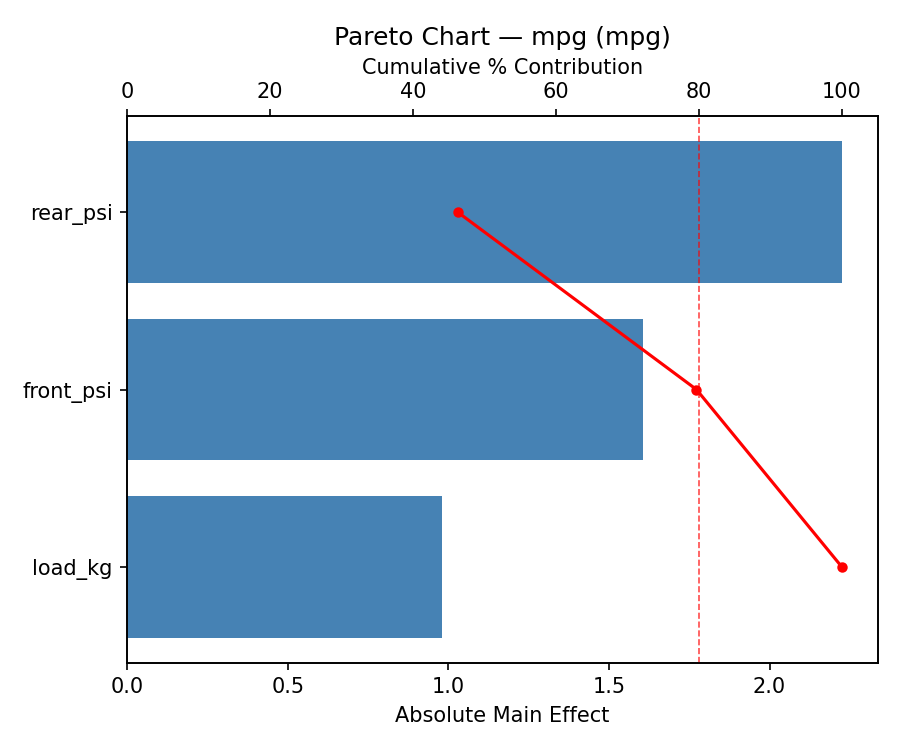
Response: mpg

Top factors: rear_psi (47.8%), front_psi (38.3%), load_kg (13.9%).

ANOVA

Source	DF	SS	MS	F	p-value
Source	DF	SS	MS	F	p-value
front_psi	2	13.1639	6.5819	1.033	0.3989
rear_psi	2	26.8899	13.4450	2.111	0.1836
load_kg	2	1.9014	0.9507	0.149	0.8637
Lack	of	Fit	6	27.4409	4.5735
Pure	Error	2	12.7400
Error	8	40.1809	6.3700
Total	14	82.1360	5.8669

Pareto Chart

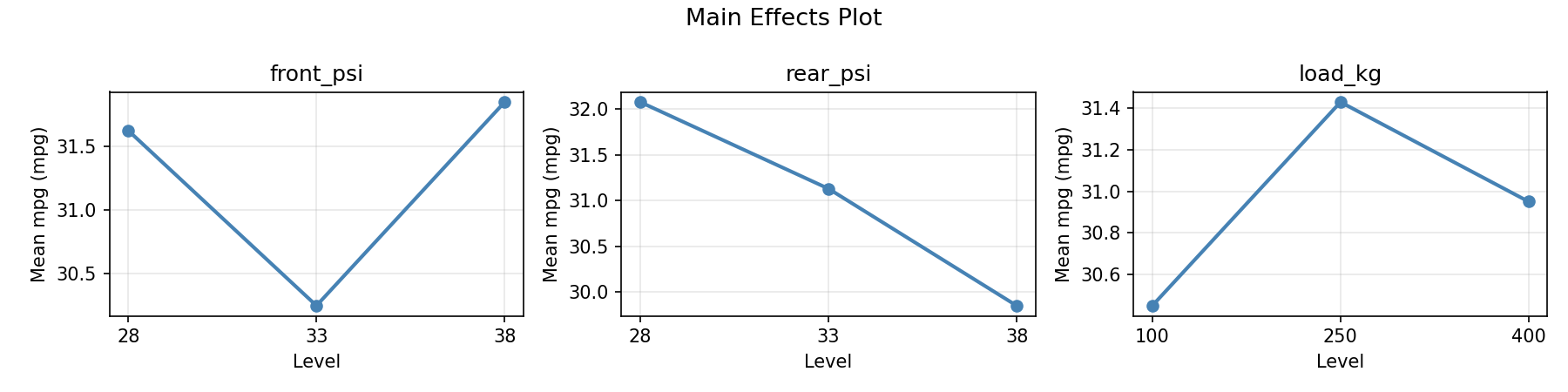
Main Effects Plot

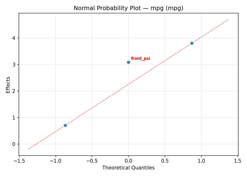
Normal Probability Plot of Effects

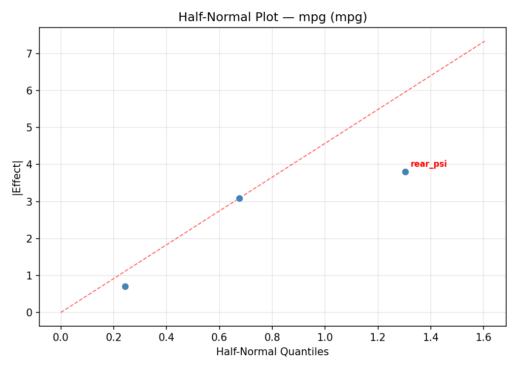
Half-Normal Plot of Effects

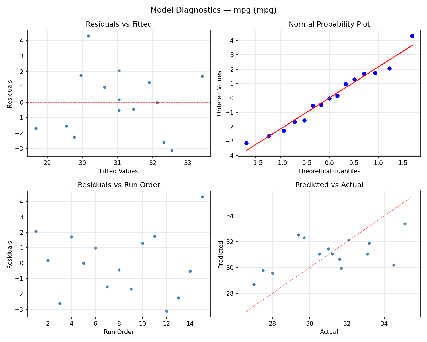
Model Diagnostics

Response: wear_rate

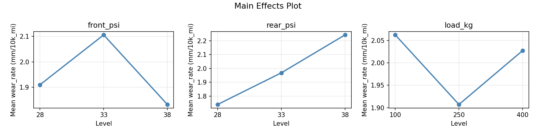
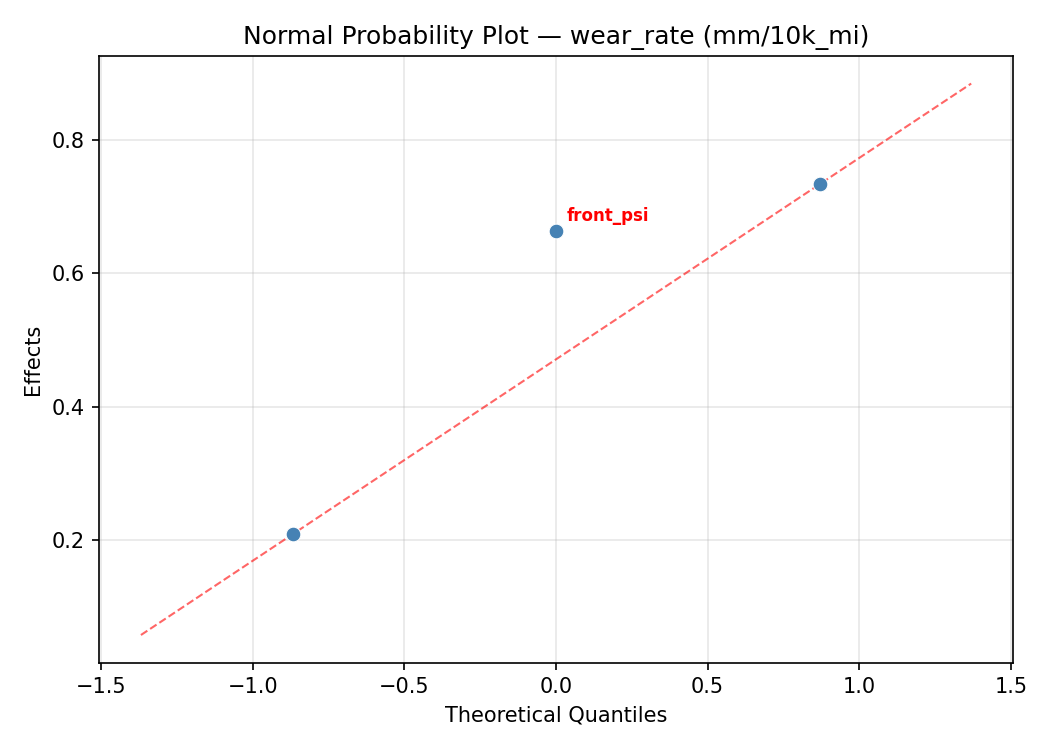
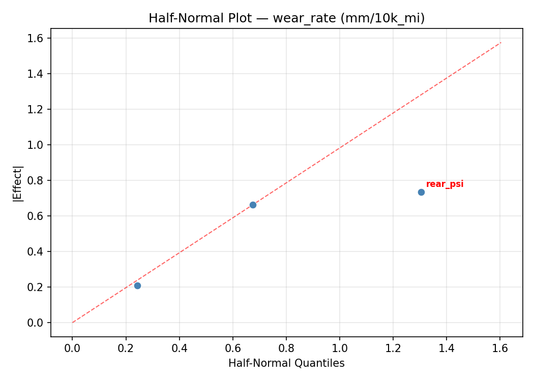
Top factors: rear_psi (43.6%), front_psi (34.4%), load_kg (22.0%).

ANOVA

Source	DF	SS	MS	F	p-value
Source	DF	SS	MS	F	p-value
front_psi	2	0.4776	0.2388	0.980	0.4162
rear_psi	2	1.0462	0.5231	2.146	0.1794
load_kg	2	0.1904	0.0952	0.391	0.6889
Lack	of	Fit	6	1.3041	0.2173
Pure	Error	2	0.4874
Error	8	1.7915	0.2437
Total	14	3.5057	0.2504

Pareto Chart

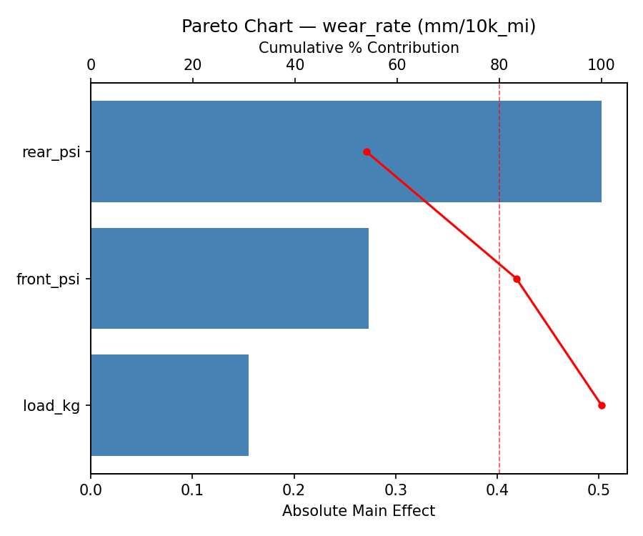
Main Effects Plot

Normal Probability Plot of Effects

Half-Normal Plot of Effects

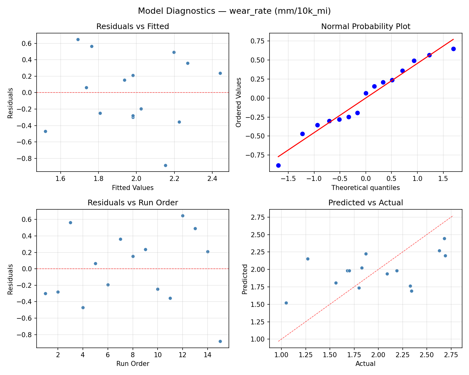
Model Diagnostics

Response Surface Plots

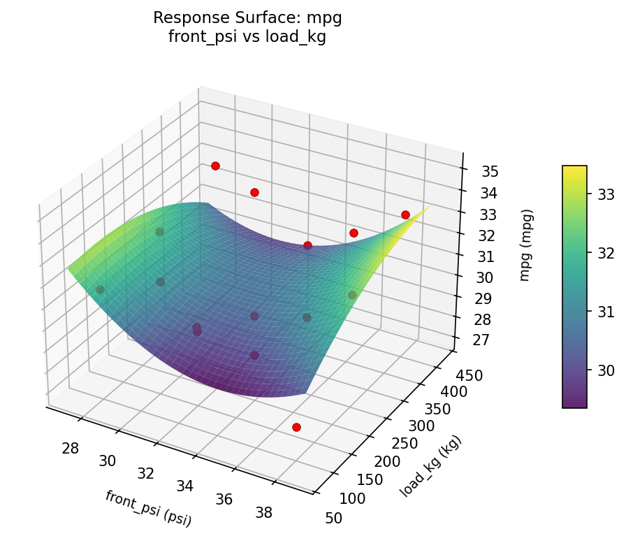
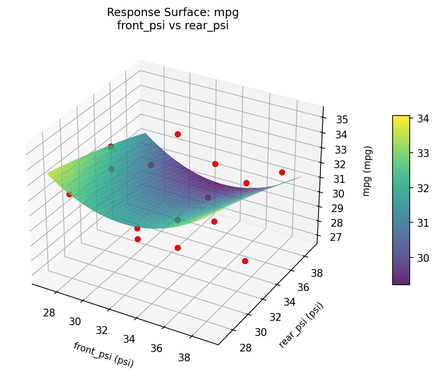
3D surfaces fitted with quadratic RSM. Red dots are observed data points.

mpg front psi vs load kg

mpg front psi vs rear psi

mpg rear psi vs load kg

wear rate front psi vs load kg

wear rate front psi vs rear psi

wear rate rear psi vs load kg

Multi-Objective Optimization

When responses compete, Derringer–Suich desirability finds the best compromise. Each response is scaled to a 0–1 desirability, then combined via a weighted geometric mean.

Overall Desirability

D = 1.0000

Per-Response Desirability

Response	Weight	Desirability	Predicted	Dir
`mpg`	1.5	1.0000	35.72 1.0000 35.72 mpg	↑
`wear_rate`	1.0	1.0000	0.95 1.0000 0.95 mm/10k_mi	↓

Recommended Settings

Factor	Value
`front_psi`	28 psi
`rear_psi`	38 psi
`load_kg`	280 kg

Source: from RSM model prediction

Trade-off Summary

Sacrifice = how much worse than single-objective best.

Response	Predicted	Best Observed	Sacrifice
`wear_rate`	0.95	1.05	-0.10

Top 3 Runs by Desirability

Run	D	Factor Settings
#15	0.8649	front_psi=38, rear_psi=28, load_kg=250
#10	0.7127	front_psi=28, rear_psi=33, load_kg=400

Model Quality

Response	R²	Type
`wear_rate`	0.7888	quadratic

Full Multi-Objective Output

doe optimize --multi
============================================================
MULTI-OBJECTIVE OPTIMIZATION
Method: Derringer-Suich Desirability Function
============================================================

Overall desirability: D = 1.0000

Response                  Weight Desirability    Predicted  Direction
---------------------------------------------------------------------
mpg                          1.5       1.0000       35.72 mpg   ↑
wear_rate                    1.0       1.0000        0.95 mm/10k_mi   ↓

Recommended settings:
  front_psi = 28 psi
  rear_psi = 38 psi
  load_kg = 280 kg
  (from RSM model prediction)

Trade-off summary:
  mpg: 35.72 (best observed: 35.10, sacrifice: -0.62)
  wear_rate: 0.95 (best observed: 1.05, sacrifice: -0.10)

Model quality:
  mpg: R² = 0.7003 (quadratic)
  wear_rate: R² = 0.7888 (quadratic)

Top 3 observed runs by overall desirability:
  1. Run #4 (D=0.9545): front_psi=28, rear_psi=38, load_kg=250
  2. Run #15 (D=0.8649): front_psi=38, rear_psi=28, load_kg=250
  3. Run #10 (D=0.7127): front_psi=28, rear_psi=33, load_kg=400

Full Analysis Output

doe analyze
=== Main Effects: mpg ===
Factor                   Effect    Std Error   % Contribution
--------------------------------------------------------------
rear_psi                 2.8357       0.6254            47.8%
front_psi                2.2679       0.6254            38.3%
load_kg                  0.8250       0.6254            13.9%

=== ANOVA Table: mpg ===
Source                      DF           SS           MS          F    p-value
-----------------------------------------------------------------------------
front_psi                    2      13.1639       6.5819      1.033     0.3989
rear_psi                     2      26.8899      13.4450      2.111     0.1836
load_kg                      2       1.9014       0.9507      0.149     0.8637
Lack of Fit                  6      27.4409       4.5735      0.718     0.6815
Pure Error                   2      12.7400       6.3700
Error                        8      40.1809       6.3700
Total                       14      82.1360       5.8669

=== Summary Statistics: mpg ===

front_psi:
  Level               N       Mean        Std        Min        Max
  ------------------------------------------------------------
  28                  4    32.5250     0.7411    31.7000    33.2000
  33                  7    30.2571     2.5475    27.0000    34.5000
  38                  4    30.9250     3.0761    28.0000    35.1000

rear_psi:
  Level               N       Mean        Std        Min        Max
  ------------------------------------------------------------
  28                  4    32.4500     2.1205    30.5000    35.1000
  33                  7    29.6143     2.1767    27.0000    32.1000
  38                  4    32.1250     2.1077    29.7000    34.5000

load_kg:
  Level               N       Mean        Std        Min        Max
  ------------------------------------------------------------
  100                 4    31.2750     2.7330    28.0000    34.5000
  250                 7    31.2429     3.0082    27.0000    35.1000
  400                 4    30.4500     1.0847    29.4000    31.7000

=== Main Effects: wear_rate ===
Factor                   Effect    Std Error   % Contribution
--------------------------------------------------------------
rear_psi                 0.5404       0.1292            43.6%
front_psi                0.4268       0.1292            34.4%
load_kg                  0.2732       0.1292            22.0%

=== ANOVA Table: wear_rate ===
Source                      DF           SS           MS          F    p-value
-----------------------------------------------------------------------------
front_psi                    2       0.4776       0.2388      0.980     0.4162
rear_psi                     2       1.0462       0.5231      2.146     0.1794
load_kg                      2       0.1904       0.0952      0.391     0.6889
Lack of Fit                  6       1.3041       0.2173      0.892     0.6143
Pure Error                   2       0.4874       0.2437
Error                        8       1.7915       0.2437
Total                       14       3.5057       0.2504

=== Summary Statistics: wear_rate ===

front_psi:
  Level               N       Mean        Std        Min        Max
  ------------------------------------------------------------
  28                  4     1.7275     0.1365     1.5600     1.8700
  33                  7     2.1543     0.4978     1.2700     2.6900
  38                  4     1.9300     0.7037     1.0500     2.6300

rear_psi:
  Level               N       Mean        Std        Min        Max
  ------------------------------------------------------------
  28                  4     1.7225     0.5267     1.0500     2.1900
  33                  7     2.2629     0.4190     1.8000     2.6900
  38                  4     1.7450     0.4375     1.2700     2.3300

load_kg:
  Level               N       Mean        Std        Min        Max
  ------------------------------------------------------------
  100                 4     1.9725     0.5782     1.2700     2.6300
  250                 7     1.8843     0.6003     1.0500     2.6900
  400                 4     2.1575     0.2238     1.8700     2.3400

Optimization Recommendations

doe optimize
=== Optimization: mpg ===
Direction: maximize

Best observed run: #4
  front_psi = 33
  rear_psi = 38
  load_kg = 400
  Value: 35.1

RSM Model (linear, R² = 0.3977, Adj R² = 0.2335):
  Coefficients:
    intercept                      +31.0400
    front_psi                      -0.2250
    rear_psi                       +0.6125
    load_kg                        -1.9125

RSM Model (quadratic, R² = 0.8489, Adj R² = 0.5770):
  Coefficients:
    intercept                      +31.5000
    front_psi                      -0.2250
    rear_psi                       +0.6125
    load_kg                        -1.9125
    front_psi*rear_psi             -0.2000
    front_psi*load_kg              +0.1000
    rear_psi*load_kg               +2.3750
    front_psi^2                    -1.7875
    rear_psi^2                     +0.4375
    load_kg^2                      +0.4875

  Curvature analysis:
    front_psi                      coef=-1.7875  concave (has a maximum)
    load_kg                        coef=+0.4875  convex (has a minimum)
    rear_psi                       coef=+0.4375  convex (has a minimum)

  Notable interactions:
    rear_psi*load_kg               coef=+2.3750  (synergistic)

  Predicted optimum (from quadratic model, at observed points):
    front_psi = 33
    rear_psi = 28
    load_kg = 100
    Predicted value: 36.1000

  Surface optimum (via L-BFGS-B, quadratic model):
    front_psi = 32.8252
    rear_psi = 28
    load_kg = 100
    Predicted value: 36.1022

  Model quality: Good fit — general trends are captured, some noise remains.

Factor importance:
  1. load_kg  (effect: 3.8, contribution: 53.7%)
  2. front_psi  (effect: 2.1, contribution: 29.2%)
  3. rear_psi  (effect: 1.2, contribution: 17.2%)

=== Optimization: wear_rate ===
Direction: minimize

Best observed run: #4
  front_psi = 33
  rear_psi = 38
  load_kg = 400
  Value: 1.05

RSM Model (linear, R² = 0.3168, Adj R² = 0.1305):
  Coefficients:
    intercept                      +1.9807
    front_psi                      +0.0350
    rear_psi                       -0.1425
    load_kg                        +0.3425

RSM Model (quadratic, R² = 0.8713, Adj R² = 0.6397):
  Coefficients:
    intercept                      +1.8000
    front_psi                      +0.0350
    rear_psi                       -0.1425
    load_kg                        +0.3425
    front_psi*rear_psi             +0.0275
    front_psi*load_kg              +0.0325
    rear_psi*load_kg               -0.5275
    front_psi^2                    +0.4513
    rear_psi^2                     -0.0138
    load_kg^2                      -0.0988

  Curvature analysis:
    front_psi                      coef=+0.4513  convex (has a minimum)
    load_kg                        coef=-0.0988  negligible curvature
    rear_psi                       coef=-0.0138  negligible curvature

  Notable interactions:
    rear_psi*load_kg               coef=-0.5275  (antagonistic)

  Predicted optimum (from quadratic model, at observed points):
    front_psi = 33
    rear_psi = 28
    load_kg = 400
    Predicted value: 2.7000

  Surface optimum (via L-BFGS-B, quadratic model):
    front_psi = 33.1385
    rear_psi = 28
    load_kg = 100
    Predicted value: 0.9597

  Model quality: Good fit — general trends are captured, some noise remains.

Factor importance:
  1. load_kg  (effect: 0.7, contribution: 46.8%)
  2. front_psi  (effect: 0.5, contribution: 33.8%)
  3. rear_psi  (effect: 0.3, contribution: 19.5%)

Run	`front_psi`	`rear_psi`	`load_kg`
1	33	28	100
2	33	33	250
3	38	33	400
4	38	33	100
5	33	33	250
6	33	33	250
7	28	33	400
8	38	28	250
9	33	28	400
10	38	38	250
11	28	33	100
12	33	38	400
13	28	28	250
14	28	38	250
15	33	38	100

Run	`front_psi`	`rear_psi`	`load_kg`
1	33	28	100
2	33	33	250
3	38	33	400
4	38	33	100
5	33	33	250
6	33	33	250
7	28	33	400
8	38	28	250
9	33	28	400
10	38	38	250
11	28	33	100
12	33	38	400
13	28	28	250
14	28	38	250
15	33	38	100

Run	`front_psi`	`rear_psi`	`load_kg`
1	33	28	100
2	33	33	250
3	38	33	400
4	38	33	100
5	33	33	250
6	33	33	250
7	28	33	400
8	38	28	250
9	33	28	400
10	38	38	250
11	28	33	100
12	33	38	400
13	28	28	250
14	28	38	250
15	33	38	100