Summary
This experiment investigates engine oil change interval. Central composite design to maximize engine longevity and minimize cost by tuning oil viscosity, change interval, and filter quality.
The design varies 3 factors: viscosity w (W), ranging from 0 to 10, change interval (miles), ranging from 3000 to 10000, and filter quality (tier), ranging from 1 to 5. The goal is to optimize 2 responses: engine health (pts) (maximize) and annual cost (USD) (minimize). Fixed conditions held constant across all runs include engine type = gasoline_4cyl, driving style = mixed.
A Central Composite Design (CCD) was selected to fit a full quadratic response surface model, including curvature and interaction effects. With 3 factors this produces 22 runs including center points and axial (star) points that extend beyond the factorial range.
Quadratic response surface models were fitted to capture potential curvature and factor interactions. The RSM contour plots below visualize how pairs of factors jointly affect each response.
Key Findings
For engine health, the most influential factors were change interval (56.3%), filter quality (23.9%), viscosity w (19.8%). The best observed value was 89.0 (at viscosity w = 5, change interval = 109.903, filter quality = 3).
For annual cost, the most influential factors were change interval (53.2%), viscosity w (23.6%), filter quality (23.2%). The best observed value was 58.0 (at viscosity w = 5, change interval = 6500, filter quality = -0.651484).
Recommended Next Steps
- Run confirmation experiments at the predicted optimal settings to validate the model.
- Consider whether any fixed factors should be varied in a future study.
Experimental Setup
Factors
| Factor | Low | High | Unit |
|---|
viscosity_w | 0 | 10 | W |
change_interval | 3000 | 10000 | miles |
filter_quality | 1 | 5 | tier |
Fixed: engine_type = gasoline_4cyl, driving_style = mixed
Responses
| Response | Direction | Unit |
|---|
engine_health | ↑ maximize | pts |
annual_cost | ↓ minimize | USD |
Configuration
{
"metadata": {
"name": "Engine Oil Change Interval",
"description": "Central composite design to maximize engine longevity and minimize cost by tuning oil viscosity, change interval, and filter quality"
},
"factors": [
{
"name": "viscosity_w",
"levels": [
"0",
"10"
],
"type": "continuous",
"unit": "W"
},
{
"name": "change_interval",
"levels": [
"3000",
"10000"
],
"type": "continuous",
"unit": "miles"
},
{
"name": "filter_quality",
"levels": [
"1",
"5"
],
"type": "continuous",
"unit": "tier"
}
],
"fixed_factors": {
"engine_type": "gasoline_4cyl",
"driving_style": "mixed"
},
"responses": [
{
"name": "engine_health",
"optimize": "maximize",
"unit": "pts"
},
{
"name": "annual_cost",
"optimize": "minimize",
"unit": "USD"
}
],
"settings": {
"operation": "central_composite",
"test_script": "use_cases/118_engine_oil_change/sim.sh"
}
}
Experimental Matrix
The Central Composite Design produces 22 runs. Each row is one experiment with specific factor settings.
| Run | viscosity_w | change_interval | filter_quality |
|---|
| 1 | 5 | 6500 | 3 |
| 2 | 10 | 3000 | 5 |
| 3 | 0 | 10000 | 1 |
| 4 | 5 | 12890.1 | 3 |
| 5 | 5 | 6500 | 3 |
| 6 | -4.12871 | 6500 | 3 |
| 7 | 5 | 6500 | -0.651484 |
| 8 | 5 | 6500 | 3 |
| 9 | 10 | 10000 | 1 |
| 10 | 14.1287 | 6500 | 3 |
| 11 | 5 | 6500 | 3 |
| 12 | 5 | 109.903 | 3 |
| 13 | 5 | 6500 | 3 |
| 14 | 0 | 3000 | 5 |
| 15 | 5 | 6500 | 3 |
| 16 | 10 | 3000 | 1 |
| 17 | 5 | 6500 | 6.65148 |
| 18 | 10 | 10000 | 5 |
| 19 | 5 | 6500 | 3 |
| 20 | 0 | 3000 | 1 |
| 21 | 0 | 10000 | 5 |
| 22 | 5 | 6500 | 3 |
Step-by-Step Workflow
1
Preview the design
$ doe info --config use_cases/118_engine_oil_change/config.json
2
Generate the runner script
$ doe generate --config use_cases/118_engine_oil_change/config.json \
--output use_cases/118_engine_oil_change/results/run.sh --seed 42
3
Execute the experiments
$ bash use_cases/118_engine_oil_change/results/run.sh
4
Analyze results
$ doe analyze --config use_cases/118_engine_oil_change/config.json
5
Get optimization recommendations
$ doe optimize --config use_cases/118_engine_oil_change/config.json
6
Multi-objective optimization
With 2 competing responses, use --multi to find the best compromise via Derringer–Suich desirability.
$ doe optimize --config use_cases/118_engine_oil_change/config.json --multi
7
Generate the HTML report
$ doe report --config use_cases/118_engine_oil_change/config.json \
--output use_cases/118_engine_oil_change/results/report.html
Features Exercised
| Feature | Value |
|---|
| Design type | central_composite |
| Factor types | continuous (all 3) |
| Arg style | double-dash |
| Responses | 2 (engine_health ↑, annual_cost ↓) |
| Total runs | 22 |
Analysis Results
Generated from actual experiment runs using the DOE Helper Tool.
Response: engine_health
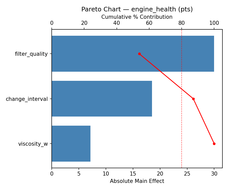
Top factors: change_interval (56.3%), filter_quality (23.9%), viscosity_w (19.8%).
ANOVA
| Source | DF | SS | MS | F | p-value |
|---|
| Source | DF | SS | MS | F | p-value |
| viscosity_w | 4 | 186.3636 | 46.5909 | 0.357 | 0.8332 |
| change_interval | 4 | 364.6970 | 91.1742 | 0.698 | 0.6121 |
| filter_quality | 4 | 203.9470 | 50.9867 | 0.390 | 0.8106 |
| Lack | of | Fit | 2 | 0.0000 | 0.0000 |
| Pure | Error | 7 | 914.0000 | | |
| Error | 9 | 903.3561 | 130.5714 | | |
| Total | 21 | 1658.3636 | 78.9697 | | |
Pareto Chart
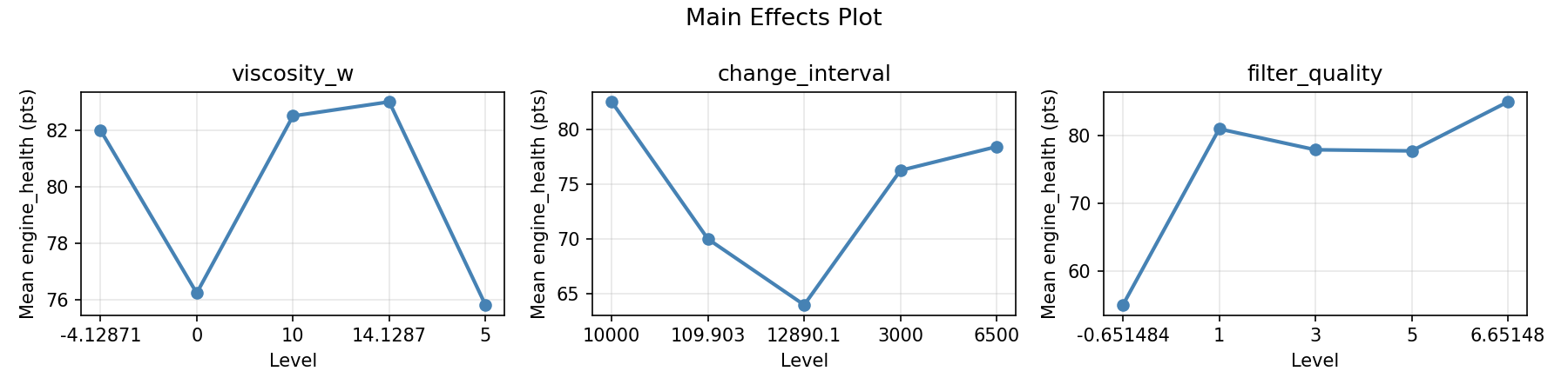
Main Effects Plot
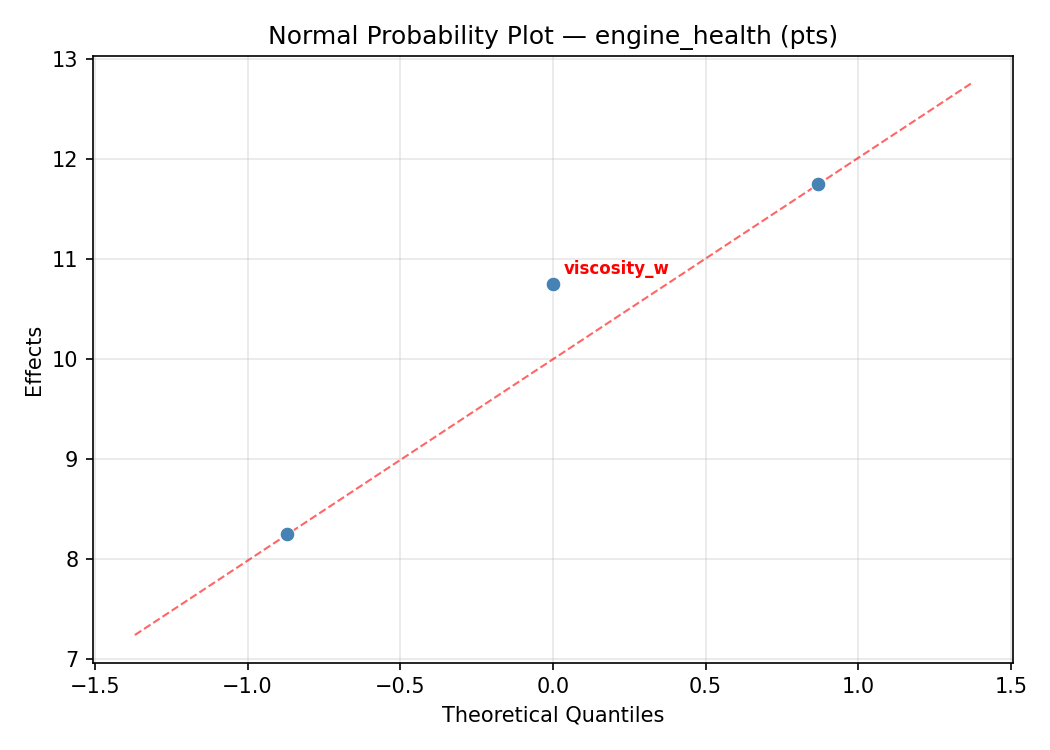
Normal Probability Plot of Effects
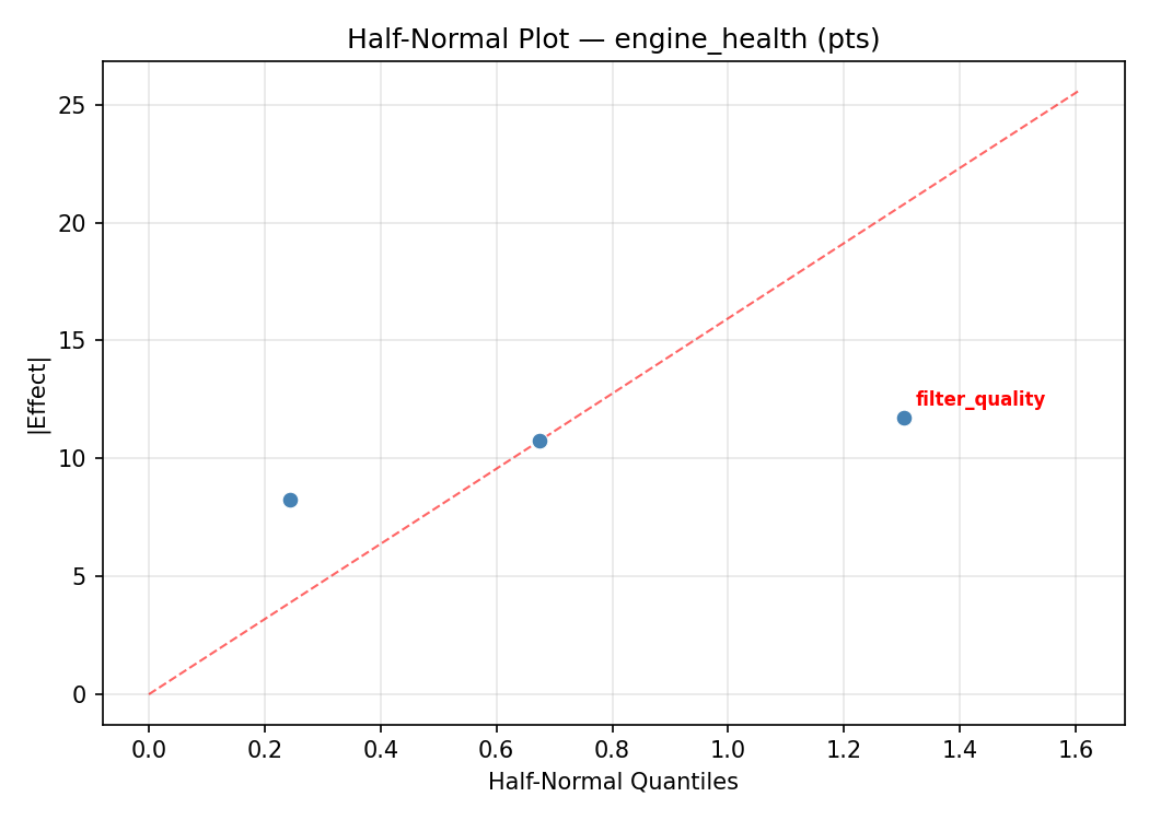
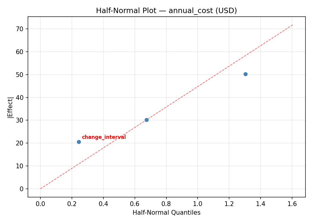
Half-Normal Plot of Effects
Model Diagnostics
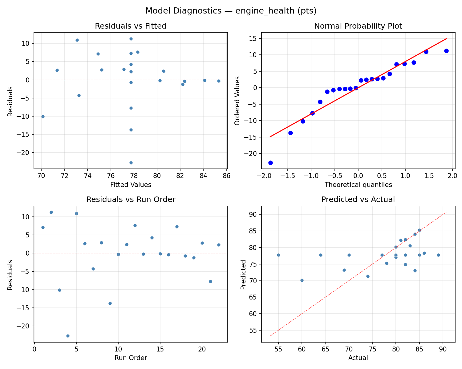
Response: annual_cost
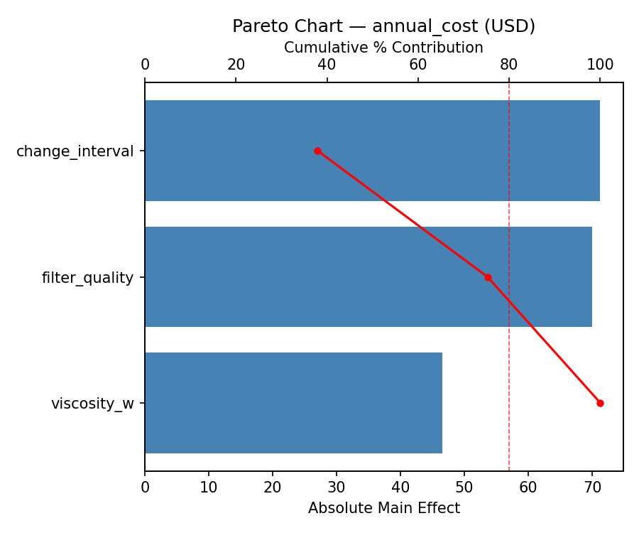
Top factors: change_interval (53.2%), viscosity_w (23.6%), filter_quality (23.2%).
ANOVA
| Source | DF | SS | MS | F | p-value |
|---|
| Source | DF | SS | MS | F | p-value |
| viscosity_w | 4 | 1603.7879 | 400.9470 | 0.184 | 0.9409 |
| change_interval | 4 | 4647.7879 | 1161.9470 | 0.533 | 0.7150 |
| filter_quality | 4 | 797.4545 | 199.3636 | 0.092 | 0.9828 |
| Lack | of | Fit | 2 | 2590.5492 | 1295.2746 |
| Pure | Error | 7 | 15249.8750 | | |
| Error | 9 | 17840.4242 | 2178.5536 | | |
| Total | 21 | 24889.4545 | 1185.2121 | | |
Pareto Chart
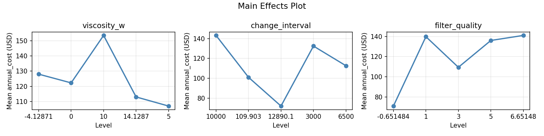
Main Effects Plot
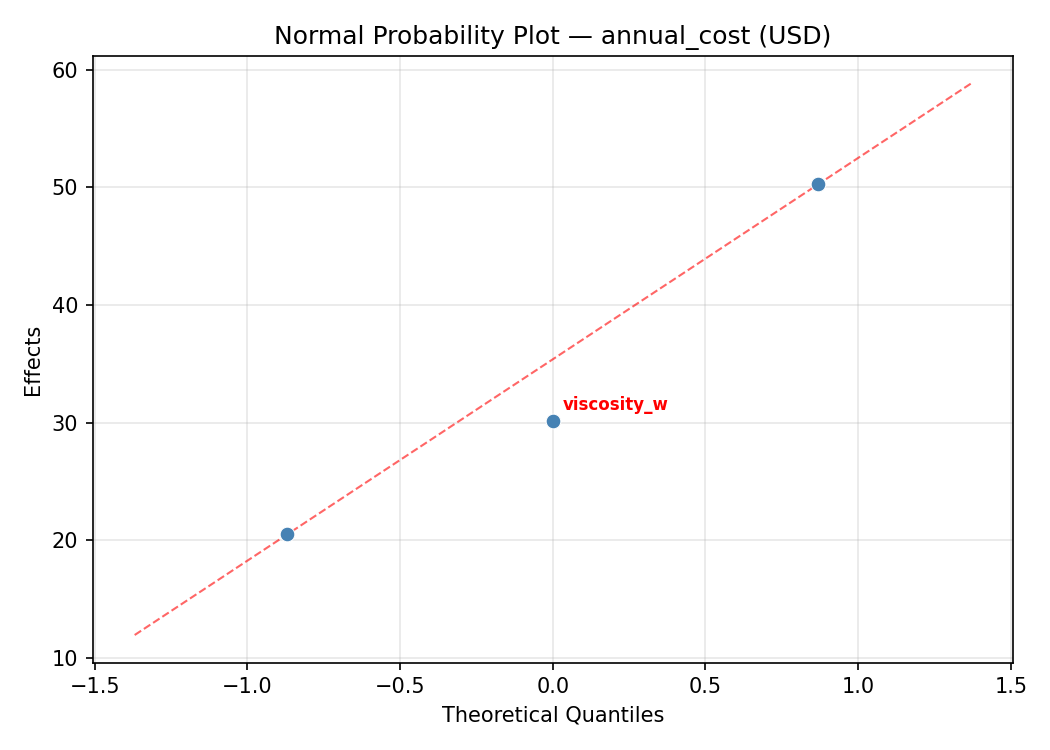
Normal Probability Plot of Effects
Half-Normal Plot of Effects
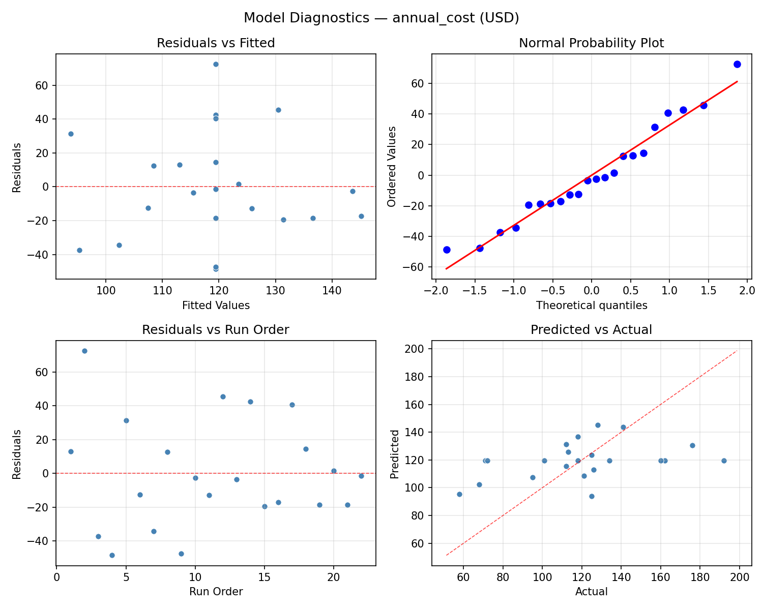
Model Diagnostics
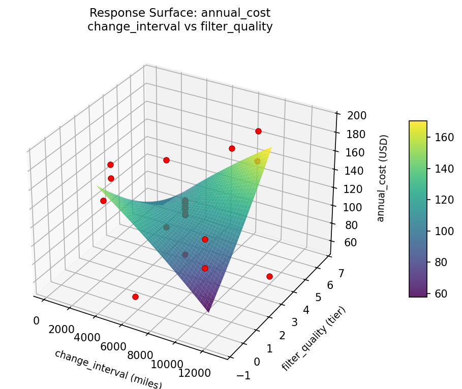
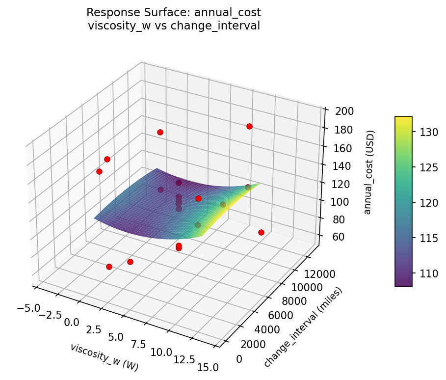
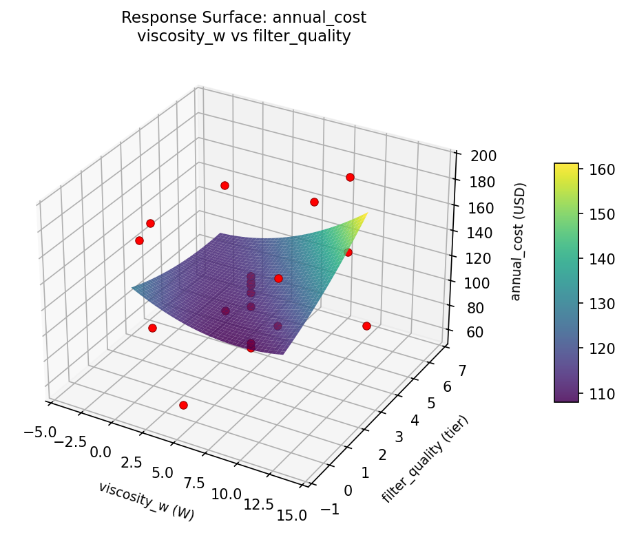
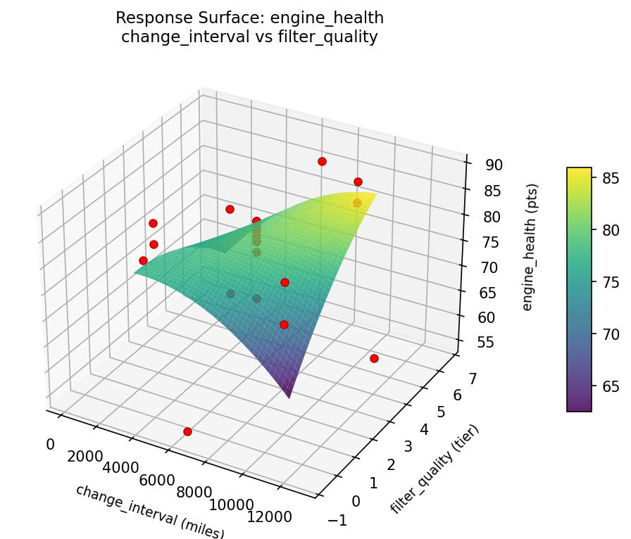
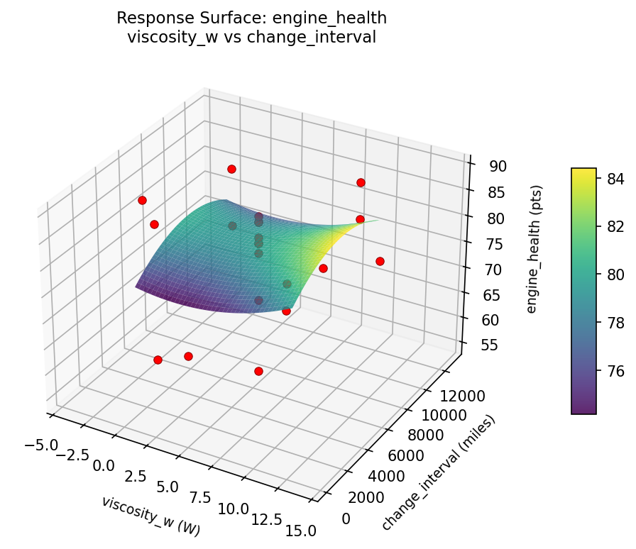
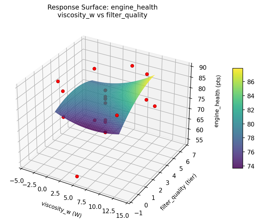
Response Surface Plots
3D surfaces fitted with quadratic RSM. Red dots are observed data points.
annual cost change interval vs filter quality
annual cost viscosity w vs change interval
annual cost viscosity w vs filter quality
engine health change interval vs filter quality
engine health viscosity w vs change interval
engine health viscosity w vs filter quality
Multi-Objective Optimization
When responses compete, Derringer–Suich desirability finds the best compromise.
Each response is scaled to a 0–1 desirability, then combined via a weighted geometric mean.
Overall Desirability
D = 0.7345
Per-Response Desirability
| Response | Weight | Desirability | Predicted | Dir |
|---|
engine_health |
2.0 |
|
84.00 0.8209 84.00 pts |
↑ |
annual_cost |
1.0 |
|
112.00 0.5882 112.00 USD |
↓ |
Recommended Settings
| Factor | Value |
|---|
viscosity_w | 10 W |
change_interval | 10000 miles |
filter_quality | 1 tier |
Source: from observed run #15
Trade-off Summary
Sacrifice = how much worse than single-objective best.
| Response | Predicted | Best Observed | Sacrifice |
|---|
annual_cost | 112.00 | 58.00 | +54.00 |
Top 3 Runs by Desirability
| Run | D | Factor Settings |
|---|
| #11 | 0.7157 | viscosity_w=5, change_interval=6500, filter_quality=3 |
| #5 | 0.6958 | viscosity_w=5, change_interval=6500, filter_quality=-0.651484 |
Model Quality
| Response | R² | Type |
|---|
annual_cost | 0.0716 | linear |
Full Multi-Objective Output
============================================================
MULTI-OBJECTIVE OPTIMIZATION
Method: Derringer-Suich Desirability Function
============================================================
Overall desirability: D = 0.7345
Response Weight Desirability Predicted Direction
---------------------------------------------------------------------
engine_health 2.0 0.8209 84.00 pts ↑
annual_cost 1.0 0.5882 112.00 USD ↓
Recommended settings:
viscosity_w = 10 W
change_interval = 10000 miles
filter_quality = 1 tier
(from observed run #15)
Trade-off summary:
engine_health: 84.00 (best observed: 89.00, sacrifice: +5.00)
annual_cost: 112.00 (best observed: 58.00, sacrifice: +54.00)
Model quality:
engine_health: R² = 0.1243 (linear)
annual_cost: R² = 0.0716 (linear)
Top 3 observed runs by overall desirability:
1. Run #15 (D=0.7345): viscosity_w=10, change_interval=10000, filter_quality=1
2. Run #11 (D=0.7157): viscosity_w=5, change_interval=6500, filter_quality=3
3. Run #5 (D=0.6958): viscosity_w=5, change_interval=6500, filter_quality=-0.651484
Full Analysis Output
=== Main Effects: engine_health ===
Factor Effect Std Error % Contribution
--------------------------------------------------------------
change_interval 22.0000 1.8946 56.3%
filter_quality 9.3333 1.8946 23.9%
viscosity_w 7.7500 1.8946 19.8%
=== ANOVA Table: engine_health ===
Source DF SS MS F p-value
-----------------------------------------------------------------------------
viscosity_w 4 186.3636 46.5909 0.357 0.8332
change_interval 4 364.6970 91.1742 0.698 0.6121
filter_quality 4 203.9470 50.9867 0.390 0.8106
Lack of Fit 2 0.0000 0.0000 0.000 1.0000
Pure Error 7 914.0000 130.5714
Error 9 903.3561 130.5714
Total 21 1658.3636 78.9697
=== Summary Statistics: engine_health ===
viscosity_w:
Level N Mean Std Min Max
------------------------------------------------------------
-4.12871 1 77.0000 0.0000 77.0000 77.0000
0 4 75.7500 7.4106 69.0000 84.0000
10 4 83.5000 1.2910 82.0000 85.0000
14.1287 1 81.0000 0.0000 81.0000 81.0000
5 12 76.2500 10.8805 55.0000 89.0000
change_interval:
Level N Mean Std Min Max
------------------------------------------------------------
10000 4 79.0000 6.9761 69.0000 85.0000
109.903 1 60.0000 0.0000 60.0000 60.0000
12890.1 1 82.0000 0.0000 82.0000 82.0000
3000 4 80.2500 6.8496 70.0000 84.0000
6500 12 77.5833 9.5675 55.0000 89.0000
filter_quality:
Level N Mean Std Min Max
------------------------------------------------------------
-0.651484 1 80.0000 0.0000 80.0000 80.0000
1 4 82.5000 1.9149 80.0000 84.0000
3 12 75.6667 10.5773 55.0000 89.0000
5 4 76.7500 8.4212 69.0000 85.0000
6.65148 1 85.0000 0.0000 85.0000 85.0000
=== Main Effects: annual_cost ===
Factor Effect Std Error % Contribution
--------------------------------------------------------------
change_interval 70.0000 7.3398 53.2%
viscosity_w 31.0000 7.3398 23.6%
filter_quality 30.5000 7.3398 23.2%
=== ANOVA Table: annual_cost ===
Source DF SS MS F p-value
-----------------------------------------------------------------------------
viscosity_w 4 1603.7879 400.9470 0.184 0.9409
change_interval 4 4647.7879 1161.9470 0.533 0.7150
filter_quality 4 797.4545 199.3636 0.092 0.9828
Lack of Fit 2 2590.5492 1295.2746 0.595 0.5774
Pure Error 7 15249.8750 2178.5536
Error 9 17840.4242 2178.5536
Total 21 24889.4545 1185.2121
=== Summary Statistics: annual_cost ===
viscosity_w:
Level N Mean Std Min Max
------------------------------------------------------------
-4.12871 1 134.0000 0.0000 134.0000 134.0000
0 4 103.0000 25.4165 68.0000 125.0000
10 4 127.7500 22.4258 112.0000 160.0000
14.1287 1 118.0000 0.0000 118.0000 118.0000
5 12 121.0833 42.4681 58.0000 192.0000
change_interval:
Level N Mean Std Min Max
------------------------------------------------------------
10000 4 118.0000 37.9825 68.0000 160.0000
109.903 1 58.0000 0.0000 58.0000 58.0000
12890.1 1 128.0000 0.0000 128.0000 128.0000
3000 4 112.7500 9.8107 101.0000 125.0000
6500 12 126.5833 37.6888 71.0000 192.0000
filter_quality:
Level N Mean Std Min Max
------------------------------------------------------------
-0.651484 1 121.0000 0.0000 121.0000 121.0000
1 4 120.2500 6.5511 112.0000 126.0000
3 12 120.2500 42.2226 58.0000 192.0000
5 4 110.5000 38.0920 68.0000 160.0000
6.65148 1 141.0000 0.0000 141.0000 141.0000
Optimization Recommendations
=== Optimization: engine_health ===
Direction: maximize
Best observed run: #2
viscosity_w = 5
change_interval = 109.903
filter_quality = 3
Value: 89.0
RSM Model (linear, R² = 0.0821, Adj R² = -0.0709):
Coefficients:
intercept +77.7273
viscosity_w +1.1560
change_interval -1.5770
filter_quality +2.3357
RSM Model (quadratic, R² = 0.8030, Adj R² = 0.6552):
Coefficients:
intercept +77.5957
viscosity_w +1.1560
change_interval -1.5770
filter_quality +2.3357
viscosity_w*change_interval +6.5000
viscosity_w*filter_quality -4.7500
change_interval*filter_quality +4.2500
viscosity_w^2 +1.5158
change_interval^2 +2.5658
filter_quality^2 -3.8842
Curvature analysis:
filter_quality coef=-3.8842 concave (has a maximum)
change_interval coef=+2.5658 convex (has a minimum)
viscosity_w coef=+1.5158 convex (has a minimum)
Notable interactions:
viscosity_w*change_interval coef=+6.5000 (synergistic)
viscosity_w*filter_quality coef=-4.7500 (antagonistic)
change_interval*filter_quality coef=+4.2500 (synergistic)
Predicted optimum (from quadratic model, at observed points):
viscosity_w = 5
change_interval = 109.903
filter_quality = 3
Predicted value: 89.0274
Surface optimum (via L-BFGS-B, quadratic model):
viscosity_w = 0
change_interval = 3000
filter_quality = 3.73007
Predicted value: 89.1158
Model quality: Good fit — general trends are captured, some noise remains.
Factor importance:
1. filter_quality (effect: 20.0, contribution: 47.1%)
2. change_interval (effect: 13.2, contribution: 31.2%)
3. viscosity_w (effect: 9.2, contribution: 21.8%)
=== Optimization: annual_cost ===
Direction: minimize
Best observed run: #3
viscosity_w = 5
change_interval = 6500
filter_quality = -0.651484
Value: 58.0
RSM Model (linear, R² = 0.1191, Adj R² = -0.0277):
Coefficients:
intercept +119.4545
viscosity_w +4.1487
change_interval -12.9586
filter_quality +4.1255
RSM Model (quadratic, R² = 0.6412, Adj R² = 0.3721):
Coefficients:
intercept +116.3230
viscosity_w +4.1487
change_interval -12.9586
filter_quality +4.1255
viscosity_w*change_interval +20.0000
viscosity_w*filter_quality -11.7500
change_interval*filter_quality +16.7500
viscosity_w^2 +7.2158
change_interval^2 +9.6158
filter_quality^2 -12.1342
Curvature analysis:
filter_quality coef=-12.1342 concave (has a maximum)
change_interval coef=+9.6158 convex (has a minimum)
viscosity_w coef=+7.2158 convex (has a minimum)
Notable interactions:
viscosity_w*change_interval coef=+20.0000 (synergistic)
change_interval*filter_quality coef=+16.7500 (synergistic)
viscosity_w*filter_quality coef=-11.7500 (antagonistic)
Predicted optimum (from quadratic model, at observed points):
viscosity_w = 5
change_interval = 109.903
filter_quality = 3
Predicted value: 172.0346
Surface optimum (via L-BFGS-B, quadratic model):
viscosity_w = 0
change_interval = 10000
filter_quality = 1
Predicted value: 51.2876
Model quality: Moderate fit — use predictions directionally, not precisely.
Factor importance:
1. change_interval (effect: 80.0, contribution: 37.4%)
2. filter_quality (effect: 69.1, contribution: 32.3%)
3. viscosity_w (effect: 65.0, contribution: 30.4%)