Summary
This experiment investigates landscape photo exposure. Box-Behnken design to maximize dynamic range and minimize noise by tuning ISO, aperture, and shutter speed.
The design varies 3 factors: iso (ISO), ranging from 100 to 3200, aperture (f-stop), ranging from 2.8 to 16, and shutter speed ms (ms), ranging from 1 to 1000. The goal is to optimize 2 responses: dynamic range ev (EV) (maximize) and noise score (pts) (minimize). Fixed conditions held constant across all runs include lens mm = 24, white balance = daylight.
A Box-Behnken design was chosen because it efficiently fits quadratic models with 3 continuous factors while avoiding extreme corner combinations — requiring only 15 runs instead of the 8 needed for a full factorial at two levels.
Quadratic response surface models were fitted to capture potential curvature and factor interactions. The RSM contour plots below visualize how pairs of factors jointly affect each response.
Key Findings
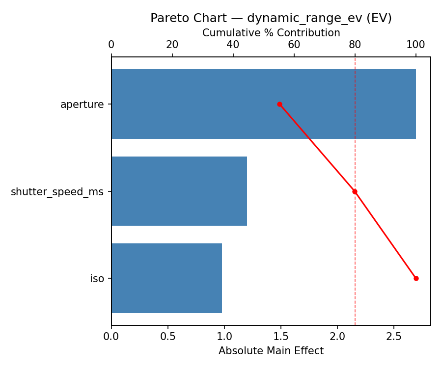
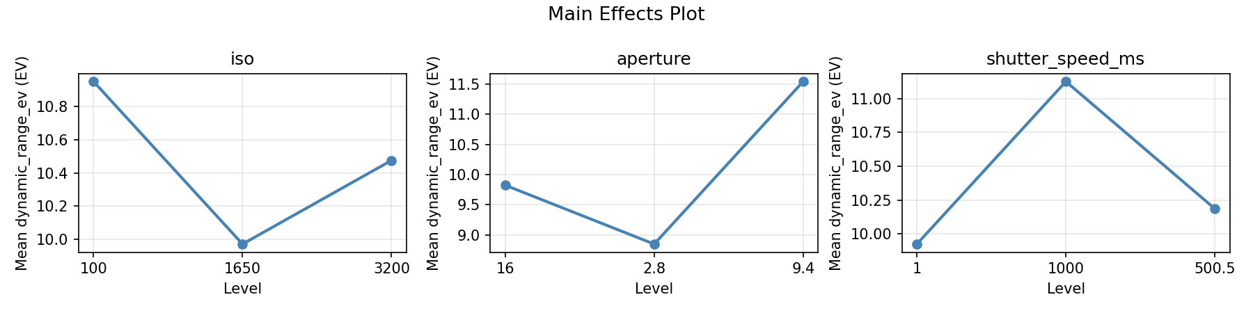
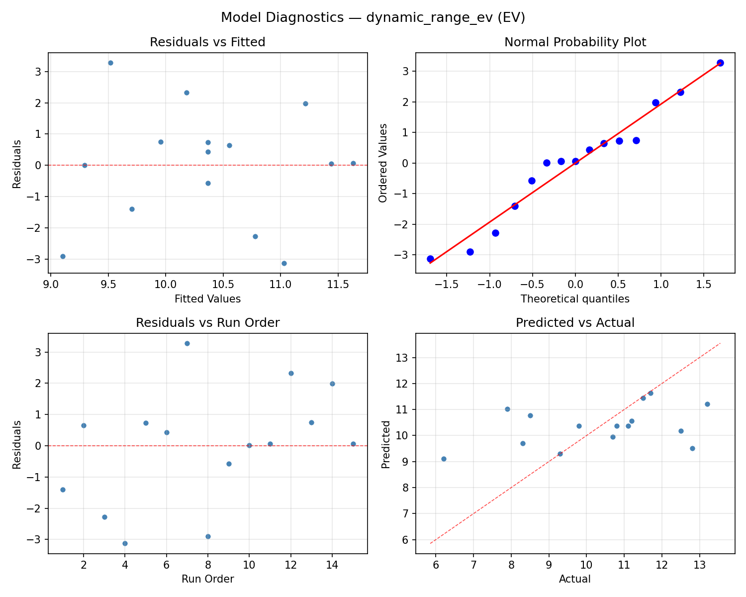
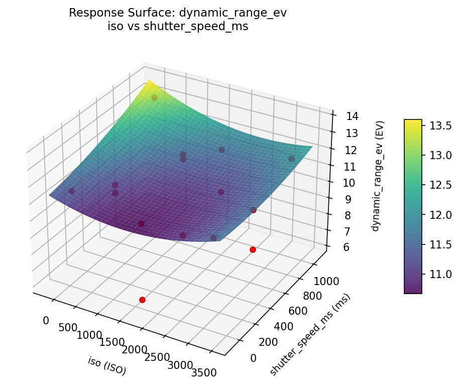
For dynamic range ev, the most influential factors were shutter speed ms (49.6%), iso (31.5%), aperture (18.9%). The best observed value was 13.2 (at iso = 1650, aperture = 9.4, shutter speed ms = 500.5).
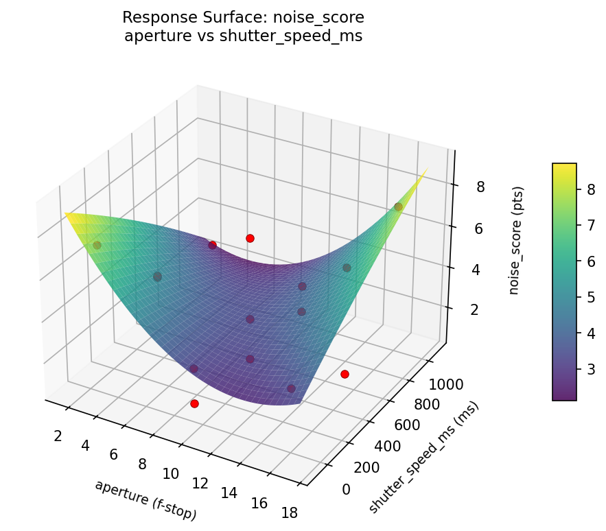
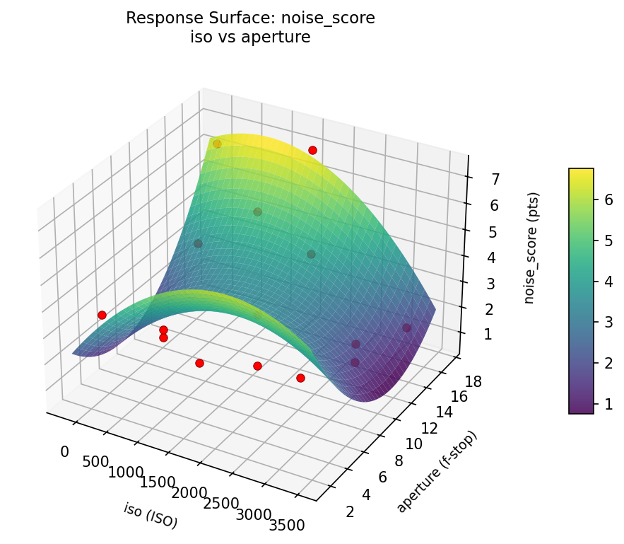
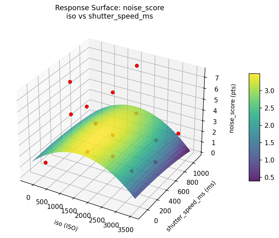
For noise score, the most influential factors were iso (54.9%), shutter speed ms (28.6%), aperture (16.6%). The best observed value was 0.8 (at iso = 1650, aperture = 2.8, shutter speed ms = 1000).
Recommended Next Steps
- Run confirmation experiments at the predicted optimal settings to validate the model.
- Consider whether any fixed factors should be varied in a future study.
Experimental Setup
Factors
| Factor | Low | High | Unit |
|---|
iso | 100 | 3200 | ISO |
aperture | 2.8 | 16 | f-stop |
shutter_speed_ms | 1 | 1000 | ms |
Fixed: lens_mm = 24, white_balance = daylight
Responses
| Response | Direction | Unit |
|---|
dynamic_range_ev | ↑ maximize | EV |
noise_score | ↓ minimize | pts |
Configuration
{
"metadata": {
"name": "Landscape Photo Exposure",
"description": "Box-Behnken design to maximize dynamic range and minimize noise by tuning ISO, aperture, and shutter speed"
},
"factors": [
{
"name": "iso",
"levels": [
"100",
"3200"
],
"type": "continuous",
"unit": "ISO"
},
{
"name": "aperture",
"levels": [
"2.8",
"16"
],
"type": "continuous",
"unit": "f-stop"
},
{
"name": "shutter_speed_ms",
"levels": [
"1",
"1000"
],
"type": "continuous",
"unit": "ms"
}
],
"fixed_factors": {
"lens_mm": "24",
"white_balance": "daylight"
},
"responses": [
{
"name": "dynamic_range_ev",
"optimize": "maximize",
"unit": "EV"
},
{
"name": "noise_score",
"optimize": "minimize",
"unit": "pts"
}
],
"settings": {
"operation": "box_behnken",
"test_script": "use_cases/147_landscape_exposure/sim.sh"
}
}
Experimental Matrix
The Box-Behnken Design produces 15 runs. Each row is one experiment with specific factor settings.
| Run | iso | aperture | shutter_speed_ms |
|---|
| 1 | 1650 | 2.8 | 1 |
| 2 | 1650 | 9.4 | 500.5 |
| 3 | 3200 | 9.4 | 1000 |
| 4 | 3200 | 9.4 | 1 |
| 5 | 1650 | 9.4 | 500.5 |
| 6 | 1650 | 9.4 | 500.5 |
| 7 | 100 | 9.4 | 1000 |
| 8 | 3200 | 2.8 | 500.5 |
| 9 | 1650 | 2.8 | 1000 |
| 10 | 3200 | 16 | 500.5 |
| 11 | 100 | 9.4 | 1 |
| 12 | 1650 | 16 | 1000 |
| 13 | 100 | 2.8 | 500.5 |
| 14 | 100 | 16 | 500.5 |
| 15 | 1650 | 16 | 1 |
Step-by-Step Workflow
1
Preview the design
$ doe info --config use_cases/147_landscape_exposure/config.json
2
Generate the runner script
$ doe generate --config use_cases/147_landscape_exposure/config.json \
--output use_cases/147_landscape_exposure/results/run.sh --seed 42
3
Execute the experiments
$ bash use_cases/147_landscape_exposure/results/run.sh
4
Analyze results
$ doe analyze --config use_cases/147_landscape_exposure/config.json
5
Get optimization recommendations
$ doe optimize --config use_cases/147_landscape_exposure/config.json
6
Multi-objective optimization
With 2 competing responses, use --multi to find the best compromise via Derringer–Suich desirability.
$ doe optimize --config use_cases/147_landscape_exposure/config.json --multi
7
Generate the HTML report
$ doe report --config use_cases/147_landscape_exposure/config.json \
--output use_cases/147_landscape_exposure/results/report.html
Features Exercised
| Feature | Value |
|---|
| Design type | box_behnken |
| Factor types | continuous (all 3) |
| Arg style | double-dash |
| Responses | 2 (dynamic_range_ev ↑, noise_score ↓) |
| Total runs | 15 |
Analysis Results
Generated from actual experiment runs using the DOE Helper Tool.
Response: dynamic_range_ev
Top factors: shutter_speed_ms (49.6%), iso (31.5%), aperture (18.9%).
ANOVA
| Source | DF | SS | MS | F | p-value |
|---|
| Source | DF | SS | MS | F | p-value |
| iso | 2 | 6.0873 | 3.0436 | 1.951 | 0.2041 |
| aperture | 2 | 1.2015 | 0.6008 | 0.385 | 0.6923 |
| shutter_speed_ms | 2 | 12.5490 | 6.2745 | 4.022 | 0.0618 |
| Lack | of | Fit | 6 | 32.7955 | 5.4659 |
| Pure | Error | 2 | 3.1200 | | |
| Error | 8 | 35.9155 | 1.5600 | | |
| Total | 14 | 55.7533 | 3.9824 | | |
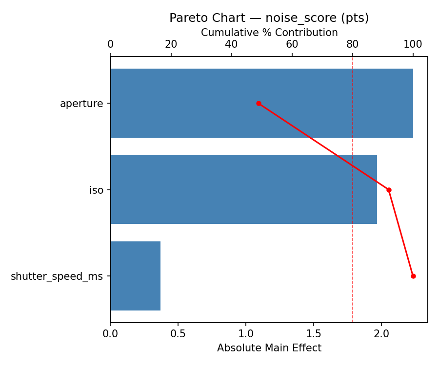
Pareto Chart
Main Effects Plot
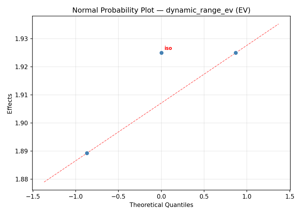
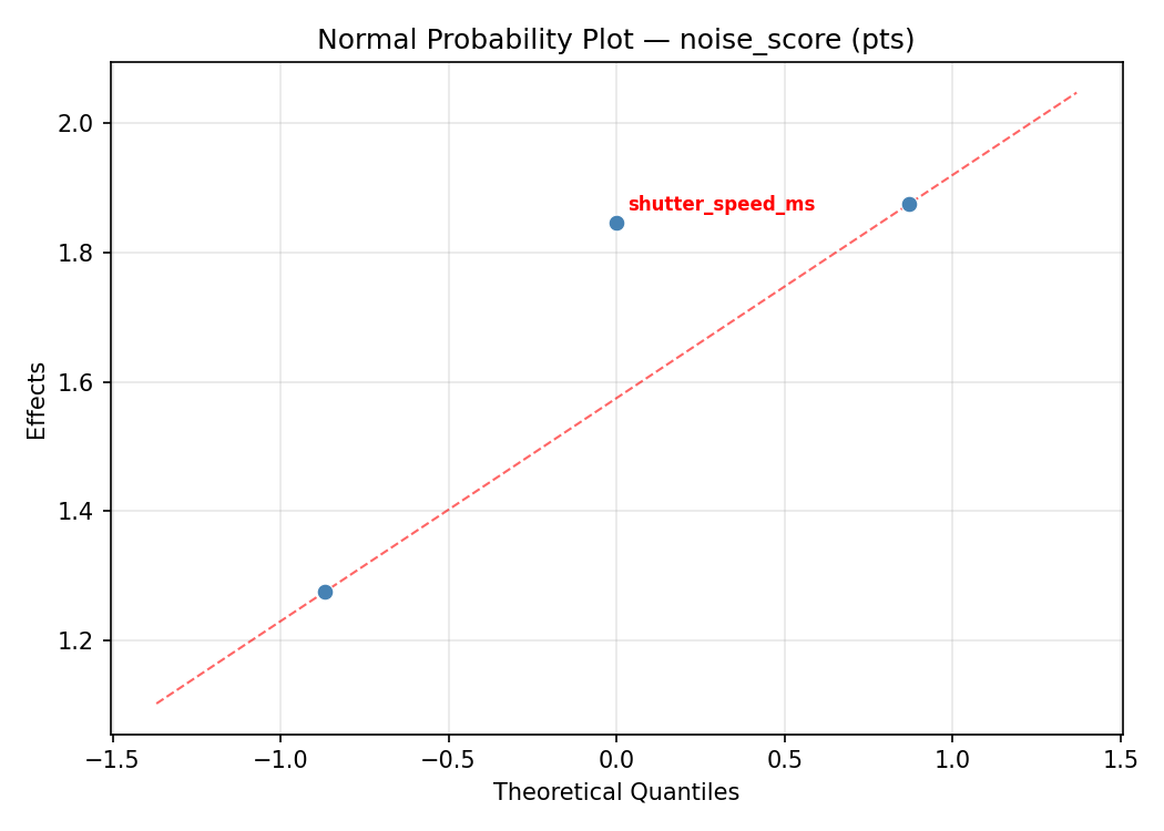
Normal Probability Plot of Effects
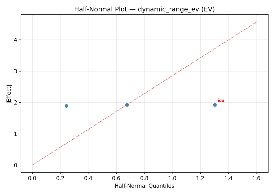
Half-Normal Plot of Effects
Model Diagnostics
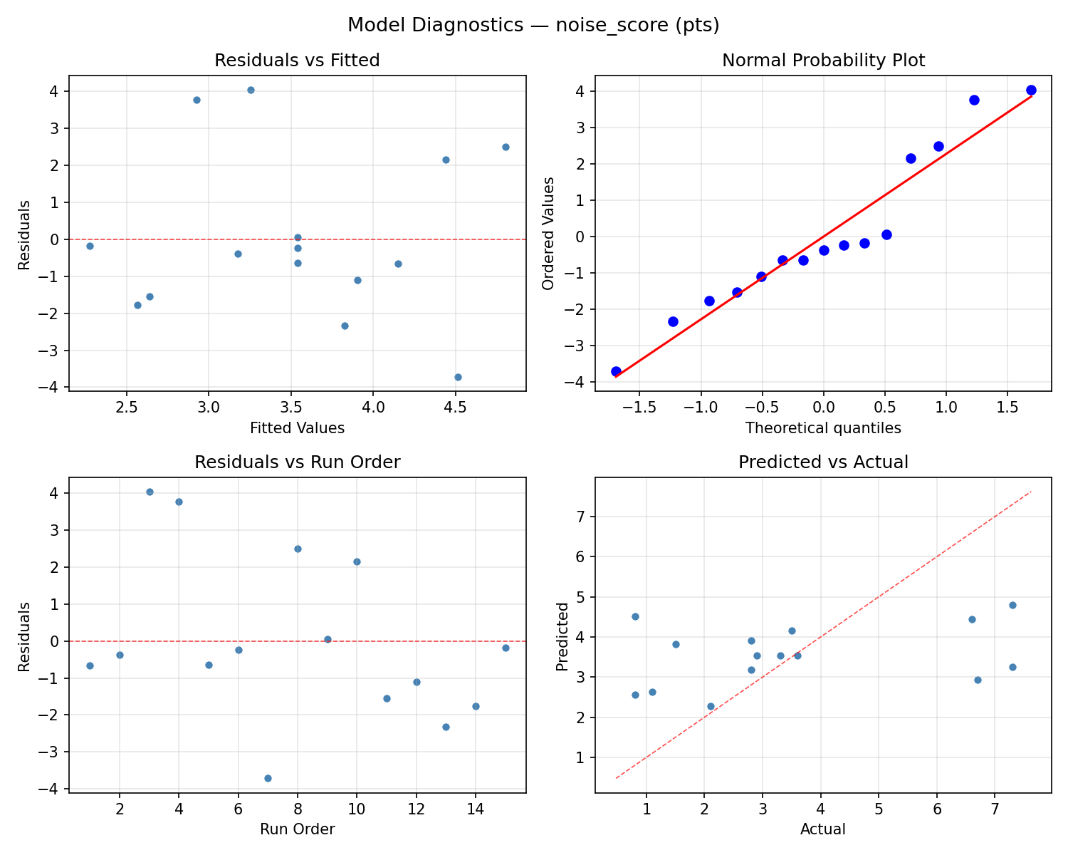
Response: noise_score
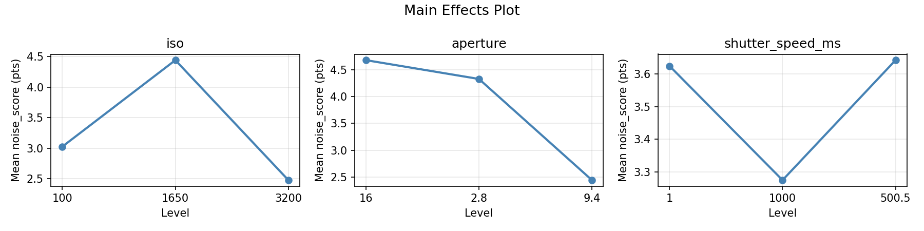
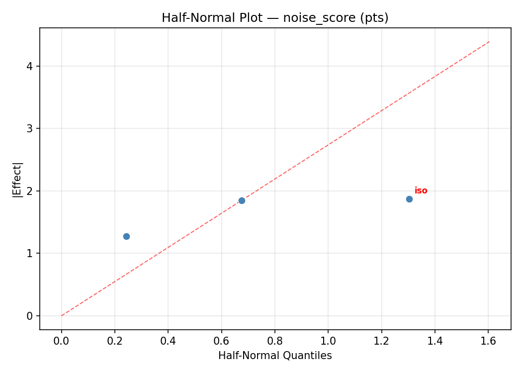
Top factors: iso (54.9%), shutter_speed_ms (28.6%), aperture (16.6%).
ANOVA
| Source | DF | SS | MS | F | p-value |
|---|
| Source | DF | SS | MS | F | p-value |
| iso | 2 | 17.5814 | 8.7907 | 1.525 | 0.2747 |
| aperture | 2 | 1.4374 | 0.7187 | 0.125 | 0.8844 |
| shutter_speed_ms | 2 | 6.1214 | 3.0607 | 0.531 | 0.6074 |
| Lack | of | Fit | 6 | 39.7292 | 6.6215 |
| Pure | Error | 2 | 11.5267 | | |
| Error | 8 | 51.2559 | 5.7633 | | |
| Total | 14 | 76.3960 | 5.4569 | | |
Pareto Chart
Main Effects Plot
Normal Probability Plot of Effects
Half-Normal Plot of Effects
Model Diagnostics
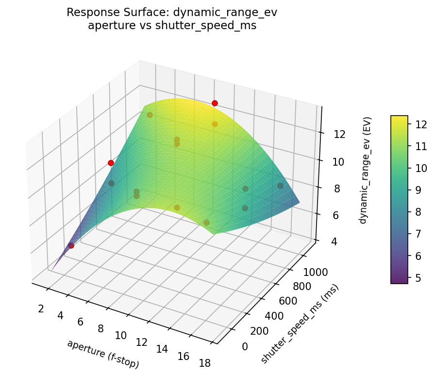
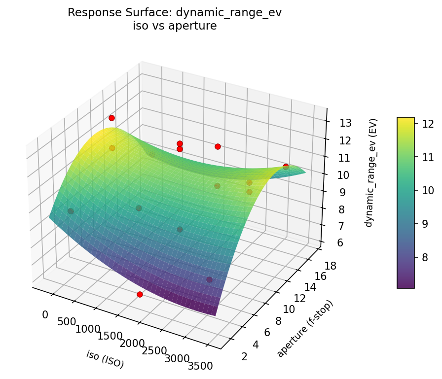
Response Surface Plots
3D surfaces fitted with quadratic RSM. Red dots are observed data points.
dynamic range ev aperture vs shutter speed ms
dynamic range ev iso vs aperture
dynamic range ev iso vs shutter speed ms
noise score aperture vs shutter speed ms
noise score iso vs aperture
noise score iso vs shutter speed ms
Multi-Objective Optimization
When responses compete, Derringer–Suich desirability finds the best compromise.
Each response is scaled to a 0–1 desirability, then combined via a weighted geometric mean.
Overall Desirability
D = 0.9545
Per-Response Desirability
| Response | Weight | Desirability | Predicted | Dir |
|---|
dynamic_range_ev |
1.5 |
|
13.20 0.9545 13.20 EV |
↑ |
noise_score |
1.0 |
|
0.80 0.9545 0.80 pts |
↓ |
Recommended Settings
| Factor | Value |
|---|
iso | 100 ISO |
aperture | 9.4 f-stop |
shutter_speed_ms | 1000 ms |
Source: from observed run #14
Trade-off Summary
Sacrifice = how much worse than single-objective best.
| Response | Predicted | Best Observed | Sacrifice |
|---|
noise_score | 0.80 | 0.80 | +0.00 |
Top 3 Runs by Desirability
| Run | D | Factor Settings |
|---|
| #7 | 0.9230 | iso=3200, aperture=9.4, shutter_speed_ms=1 |
| #11 | 0.8007 | iso=3200, aperture=9.4, shutter_speed_ms=1000 |
Model Quality
| Response | R² | Type |
|---|
noise_score | 0.2742 | linear |
Full Multi-Objective Output
============================================================
MULTI-OBJECTIVE OPTIMIZATION
Method: Derringer-Suich Desirability Function
============================================================
Overall desirability: D = 0.9545
Response Weight Desirability Predicted Direction
---------------------------------------------------------------------
dynamic_range_ev 1.5 0.9545 13.20 EV ↑
noise_score 1.0 0.9545 0.80 pts ↓
Recommended settings:
iso = 100 ISO
aperture = 9.4 f-stop
shutter_speed_ms = 1000 ms
(from observed run #14)
Trade-off summary:
dynamic_range_ev: 13.20 (best observed: 13.20, sacrifice: +0.00)
noise_score: 0.80 (best observed: 0.80, sacrifice: +0.00)
Model quality:
dynamic_range_ev: R² = 0.7624 (quadratic)
noise_score: R² = 0.2742 (linear)
Top 3 observed runs by overall desirability:
1. Run #14 (D=0.9545): iso=100, aperture=9.4, shutter_speed_ms=1000
2. Run #7 (D=0.9230): iso=3200, aperture=9.4, shutter_speed_ms=1
3. Run #11 (D=0.8007): iso=3200, aperture=9.4, shutter_speed_ms=1000
Full Analysis Output
=== Main Effects: dynamic_range_ev ===
Factor Effect Std Error % Contribution
--------------------------------------------------------------
shutter_speed_ms 2.0286 0.5153 49.6%
iso 1.2893 0.5153 31.5%
aperture 0.7750 0.5153 18.9%
=== ANOVA Table: dynamic_range_ev ===
Source DF SS MS F p-value
-----------------------------------------------------------------------------
iso 2 6.0873 3.0436 1.951 0.2041
aperture 2 1.2015 0.6008 0.385 0.6923
shutter_speed_ms 2 12.5490 6.2745 4.022 0.0618
Lack of Fit 6 32.7955 5.4659 3.504 0.2386
Pure Error 2 3.1200 1.5600
Error 8 35.9155 1.5600
Total 14 55.7533 3.9824
=== Summary Statistics: dynamic_range_ev ===
iso:
Level N Mean Std Min Max
------------------------------------------------------------
100 4 10.9750 2.2500 7.9000 12.8000
1650 7 9.6857 1.9178 6.2000 11.7000
3200 4 10.9500 2.0339 8.3000 13.2000
aperture:
Level N Mean Std Min Max
------------------------------------------------------------
16 4 9.9750 2.8987 6.2000 13.2000
2.8 4 10.7500 1.6663 8.5000 12.5000
9.4 7 10.3714 1.8715 7.9000 12.8000
shutter_speed_ms:
Level N Mean Std Min Max
------------------------------------------------------------
1 4 9.7500 2.9738 6.2000 12.8000
1000 4 9.3000 1.5078 7.9000 11.2000
500.5 7 11.3286 1.2816 9.3000 13.2000
=== Main Effects: noise_score ===
Factor Effect Std Error % Contribution
--------------------------------------------------------------
iso 2.4821 0.6032 54.9%
shutter_speed_ms 1.2929 0.6032 28.6%
aperture 0.7500 0.6032 16.6%
=== ANOVA Table: noise_score ===
Source DF SS MS F p-value
-----------------------------------------------------------------------------
iso 2 17.5814 8.7907 1.525 0.2747
aperture 2 1.4374 0.7187 0.125 0.8844
shutter_speed_ms 2 6.1214 3.0607 0.531 0.6074
Lack of Fit 6 39.7292 6.6215 1.149 0.5343
Pure Error 2 11.5267 5.7633
Error 8 51.2559 5.7633
Total 14 76.3960 5.4569
=== Summary Statistics: noise_score ===
iso:
Level N Mean Std Min Max
------------------------------------------------------------
100 4 2.9500 2.6338 0.8000 6.7000
1650 7 4.6571 2.3071 2.1000 7.3000
3200 4 2.1750 1.4221 0.8000 3.5000
aperture:
Level N Mean Std Min Max
------------------------------------------------------------
16 4 3.3000 2.9200 0.8000 7.3000
2.8 4 4.0500 2.1794 2.8000 7.3000
9.4 7 3.3857 2.4197 0.8000 6.7000
shutter_speed_ms:
Level N Mean Std Min Max
------------------------------------------------------------
1 4 4.1250 3.6682 0.8000 7.3000
1000 4 4.1500 1.7369 2.8000 6.7000
500.5 7 2.8571 1.8645 0.8000 6.6000
Optimization Recommendations
=== Optimization: dynamic_range_ev ===
Direction: maximize
Best observed run: #14
iso = 1650
aperture = 9.4
shutter_speed_ms = 500.5
Value: 13.2
RSM Model (linear, R² = 0.2882, Adj R² = 0.0941):
Coefficients:
intercept +10.3667
iso +0.4625
aperture -1.3375
shutter_speed_ms -0.0750
RSM Model (quadratic, R² = 0.6666, Adj R² = 0.0664):
Coefficients:
intercept +11.5667
iso +0.4625
aperture -1.3375
shutter_speed_ms -0.0750
iso*aperture -0.0500
iso*shutter_speed_ms -0.6750
aperture*shutter_speed_ms +0.5250
iso^2 -1.7583
aperture^2 -1.1583
shutter_speed_ms^2 +0.6667
Curvature analysis:
iso coef=-1.7583 concave (has a maximum)
aperture coef=-1.1583 concave (has a maximum)
shutter_speed_ms coef=+0.6667 convex (has a minimum)
Notable interactions:
iso*shutter_speed_ms coef=-0.6750 (antagonistic)
aperture*shutter_speed_ms coef=+0.5250 (synergistic)
Predicted optimum (from linear model, at observed points):
iso = 3200
aperture = 2.8
shutter_speed_ms = 500.5
Predicted value: 12.1667
Surface optimum (via L-BFGS-B, linear model):
iso = 3200
aperture = 2.8
shutter_speed_ms = 1
Predicted value: 12.2417
Model quality: Weak fit — consider adding center points or using a different design.
Factor importance:
1. aperture (effect: 2.7, contribution: 46.0%)
2. iso (effect: 2.2, contribution: 37.6%)
3. shutter_speed_ms (effect: 0.9, contribution: 16.3%)
=== Optimization: noise_score ===
Direction: minimize
Best observed run: #7
iso = 1650
aperture = 2.8
shutter_speed_ms = 1000
Value: 0.8
RSM Model (linear, R² = 0.1338, Adj R² = -0.1024):
Coefficients:
intercept +3.5400
iso -0.1000
aperture +1.0375
shutter_speed_ms +0.4375
RSM Model (quadratic, R² = 0.7725, Adj R² = 0.3630):
Coefficients:
intercept +1.8667
iso -0.1000
aperture +1.0375
shutter_speed_ms +0.4375
iso*aperture +0.8000
iso*shutter_speed_ms +0.9500
aperture*shutter_speed_ms -0.2750
iso^2 +3.1292
aperture^2 +0.8542
shutter_speed_ms^2 -0.8458
Curvature analysis:
iso coef=+3.1292 convex (has a minimum)
aperture coef=+0.8542 convex (has a minimum)
shutter_speed_ms coef=-0.8458 concave (has a maximum)
Notable interactions:
iso*shutter_speed_ms coef=+0.9500 (synergistic)
iso*aperture coef=+0.8000 (synergistic)
Predicted optimum (from quadratic model, at observed points):
iso = 3200
aperture = 16
shutter_speed_ms = 500.5
Predicted value: 7.5875
Surface optimum (via L-BFGS-B, quadratic model):
iso = 2088.53
aperture = 3.45483
shutter_speed_ms = 1
Predicted value: -0.1563
Model quality: Good fit — general trends are captured, some noise remains.
Factor importance:
1. iso (effect: 3.2, contribution: 47.0%)
2. aperture (effect: 2.1, contribution: 30.2%)
3. shutter_speed_ms (effect: 1.6, contribution: 22.8%)