Summary
This experiment investigates load balancer algorithm. Full factorial of balancing algorithm, health check interval, and connection draining for availability.
The design varies 3 factors: algorithm, ranging from round_robin to ip_hash, health interval (s), ranging from 5 to 30, and drain timeout (s), ranging from 10 to 60. The goal is to optimize 2 responses: availability (%) (maximize) and imbalance pct (%) (minimize). Fixed conditions held constant across all runs include backend count = 4, protocol = http2.
A full factorial design was used to explore all 8 possible combinations of the 3 factors at two levels. This guarantees that every main effect and interaction can be estimated independently, at the cost of a larger experiment (12 runs).
Quadratic response surface models were fitted to capture potential curvature and factor interactions. The RSM contour plots below visualize how pairs of factors jointly affect each response.
Key Findings
For availability, the most influential factors were algorithm (58.7%), health interval (21.3%), drain timeout (20.1%). The best observed value was 99.963 (at algorithm = least_conn, health interval = 5, drain timeout = 10).
For imbalance pct, the most influential factors were algorithm (50.1%), health interval (32.2%), drain timeout (17.7%). The best observed value was 0.1 (at algorithm = round_robin, health interval = 30, drain timeout = 10).
Recommended Next Steps
- Consider whether any fixed factors should be varied in a future study.
Experimental Setup
Factors
| Factor | Low | High | Unit |
|---|
algorithm | round_robin | ip_hash | |
health_interval | 5 | 30 | s |
drain_timeout | 10 | 60 | s |
Fixed: backend_count = 4, protocol = http2
Responses
| Response | Direction | Unit |
|---|
availability | ↑ maximize | % |
imbalance_pct | ↓ minimize | % |
Configuration
{
"metadata": {
"name": "Load Balancer Algorithm",
"description": "Full factorial of balancing algorithm, health check interval, and connection draining for availability"
},
"factors": [
{
"name": "algorithm",
"levels": [
"round_robin",
"least_conn",
"ip_hash"
],
"type": "categorical",
"unit": ""
},
{
"name": "health_interval",
"levels": [
"5",
"30"
],
"type": "continuous",
"unit": "s"
},
{
"name": "drain_timeout",
"levels": [
"10",
"60"
],
"type": "continuous",
"unit": "s"
}
],
"fixed_factors": {
"backend_count": "4",
"protocol": "http2"
},
"responses": [
{
"name": "availability",
"optimize": "maximize",
"unit": "%"
},
{
"name": "imbalance_pct",
"optimize": "minimize",
"unit": "%"
}
],
"settings": {
"operation": "full_factorial",
"test_script": "use_cases/32_load_balancer_algorithm/sim.sh"
}
}
Experimental Matrix
The Full Factorial Design produces 12 runs. Each row is one experiment with specific factor settings.
| Run | algorithm | health_interval | drain_timeout |
|---|
| 1 | least_conn | 30 | 60 |
| 2 | least_conn | 5 | 60 |
| 3 | round_robin | 30 | 10 |
| 4 | ip_hash | 5 | 10 |
| 5 | ip_hash | 5 | 60 |
| 6 | least_conn | 30 | 10 |
| 7 | ip_hash | 30 | 60 |
| 8 | round_robin | 30 | 60 |
| 9 | least_conn | 5 | 10 |
| 10 | round_robin | 5 | 10 |
| 11 | round_robin | 5 | 60 |
| 12 | ip_hash | 30 | 10 |
Step-by-Step Workflow
1
Preview the design
$ doe info --config use_cases/32_load_balancer_algorithm/config.json
2
Generate the runner script
$ doe generate --config use_cases/32_load_balancer_algorithm/config.json \
--output use_cases/32_load_balancer_algorithm/results/run.sh --seed 42
3
Execute the experiments
$ bash use_cases/32_load_balancer_algorithm/results/run.sh
4
Analyze results
$ doe analyze --config use_cases/32_load_balancer_algorithm/config.json
5
Get optimization recommendations
$ doe optimize --config use_cases/32_load_balancer_algorithm/config.json
6
Multi-objective optimization
With 2 competing responses, use --multi to find the best compromise via Derringer–Suich desirability.
$ doe optimize --config use_cases/32_load_balancer_algorithm/config.json --multi
7
Generate the HTML report
$ doe report --config use_cases/32_load_balancer_algorithm/config.json \
--output use_cases/32_load_balancer_algorithm/results/report.html
Features Exercised
| Feature | Value |
|---|
| Design type | full_factorial |
| Factor types | continuous (2), categorical (1) |
| Arg style | double-dash |
| Responses | 2 (availability ↑, imbalance_pct ↓) |
| Total runs | 12 |
Analysis Results
Generated from actual experiment runs using the DOE Helper Tool.
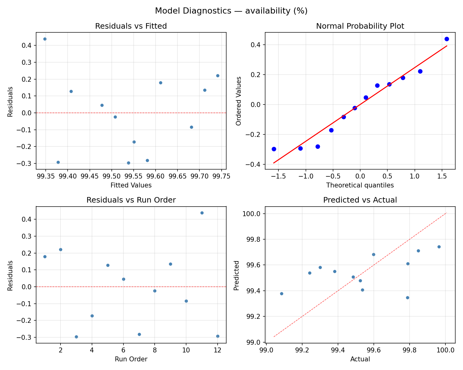
Response: availability
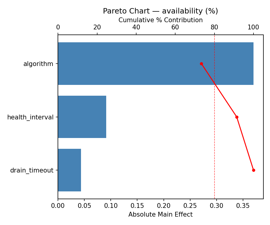
Top factors: algorithm (58.7%), health_interval (21.3%), drain_timeout (20.1%).
ANOVA
| Source | DF | SS | MS | F | p-value |
|---|
| Source | DF | SS | MS | F | p-value |
| algorithm | 2 | 0.1273 | 0.0636 | 0.619 | 0.5695 |
| health_interval | 1 | 0.0207 | 0.0207 | 0.201 | 0.6695 |
| drain_timeout | 1 | 0.0184 | 0.0184 | 0.179 | 0.6868 |
| health_interval*drain_timeout | 1 | 0.0005 | 0.0005 | 0.005 | 0.9463 |
| Error | 6 | 0.6164 | 0.1027 | | |
| Total | 11 | 0.7832 | 0.0712 | | |
Pareto Chart
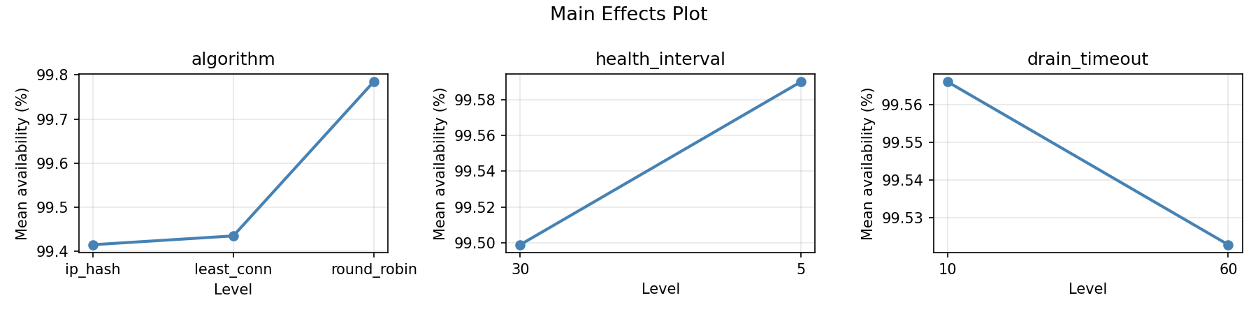
Main Effects Plot
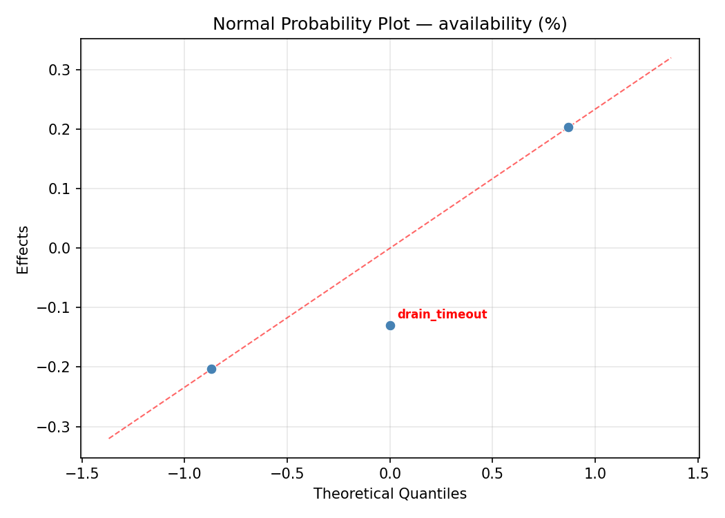
Normal Probability Plot of Effects
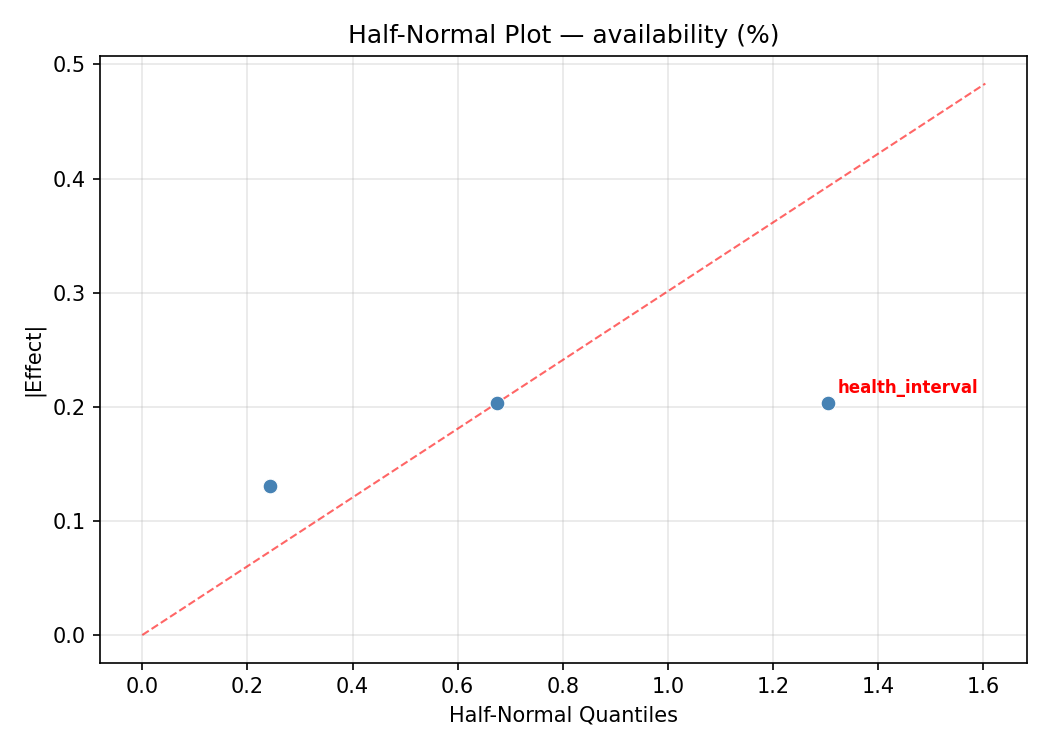
Half-Normal Plot of Effects
Model Diagnostics
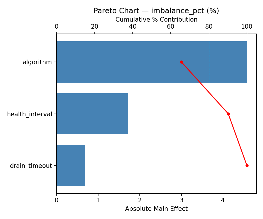
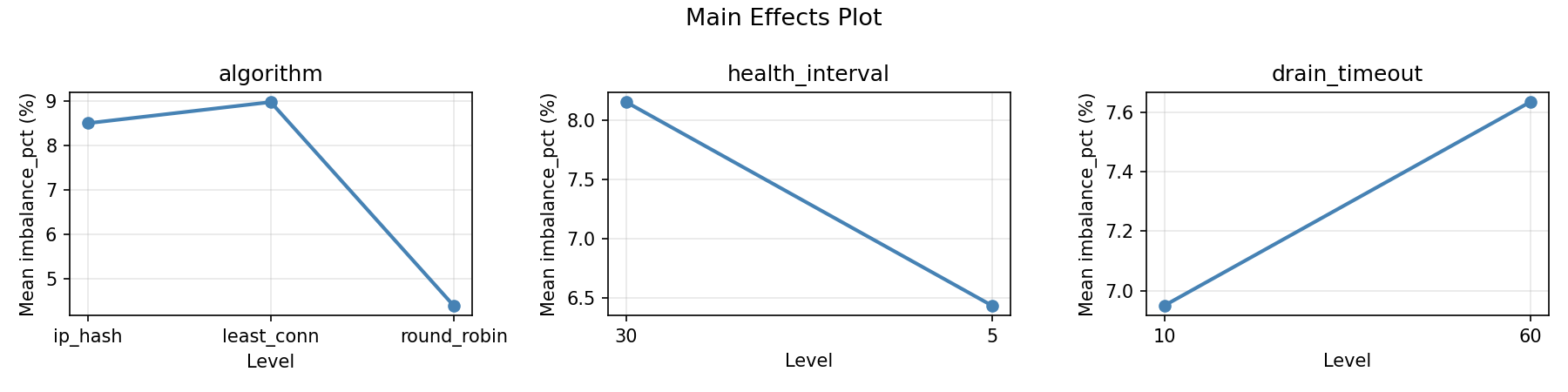
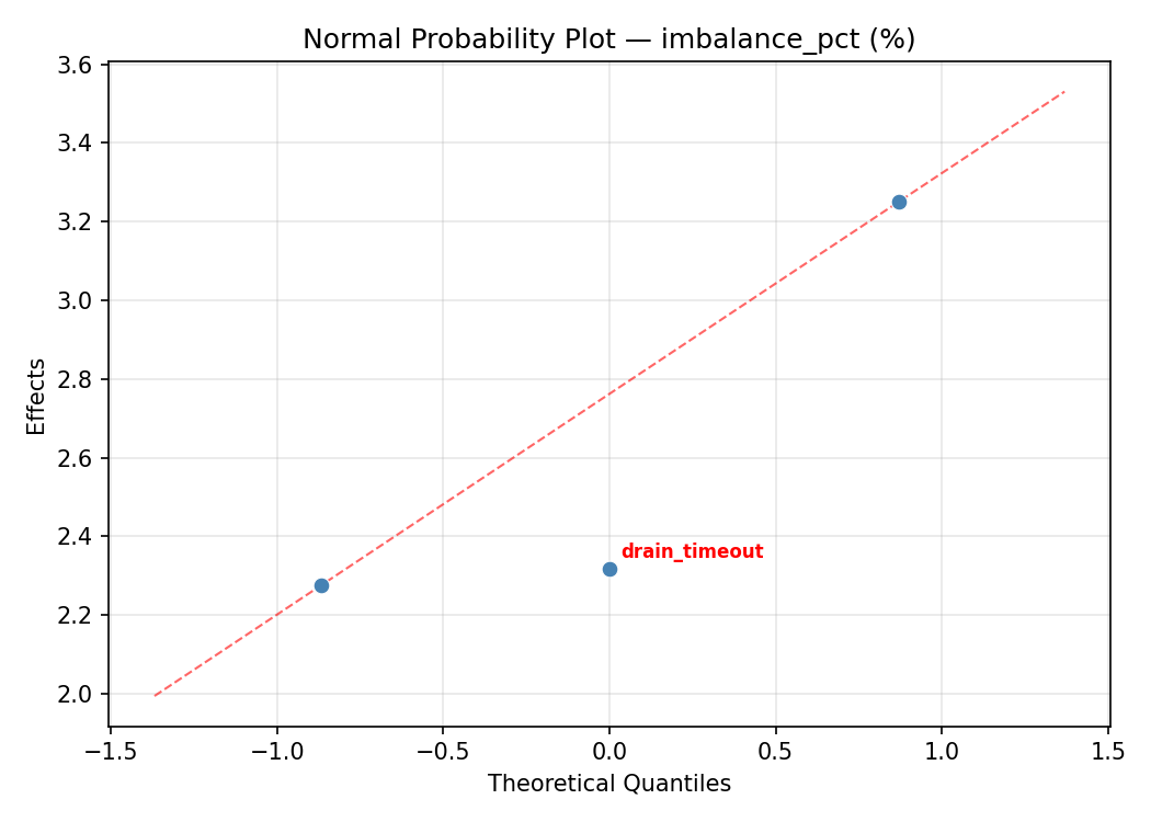
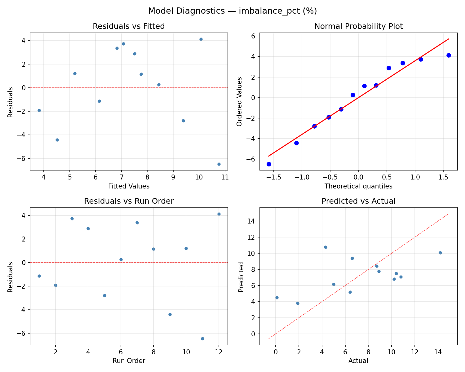
Response: imbalance_pct
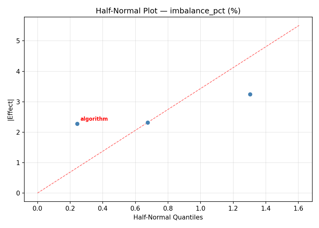
Top factors: algorithm (50.1%), health_interval (32.2%), drain_timeout (17.7%).
ANOVA
| Source | DF | SS | MS | F | p-value |
|---|
| Source | DF | SS | MS | F | p-value |
| algorithm | 2 | 26.9517 | 13.4758 | 0.606 | 0.5757 |
| health_interval | 1 | 13.8675 | 13.8675 | 0.624 | 0.4597 |
| drain_timeout | 1 | 4.2008 | 4.2008 | 0.189 | 0.6790 |
| health_interval*drain_timeout | 1 | 0.6075 | 0.6075 | 0.027 | 0.8741 |
| Error | 6 | 133.3617 | 22.2269 | | |
| Total | 11 | 178.9892 | 16.2717 | | |
Pareto Chart
Main Effects Plot
Normal Probability Plot of Effects
Half-Normal Plot of Effects
Model Diagnostics
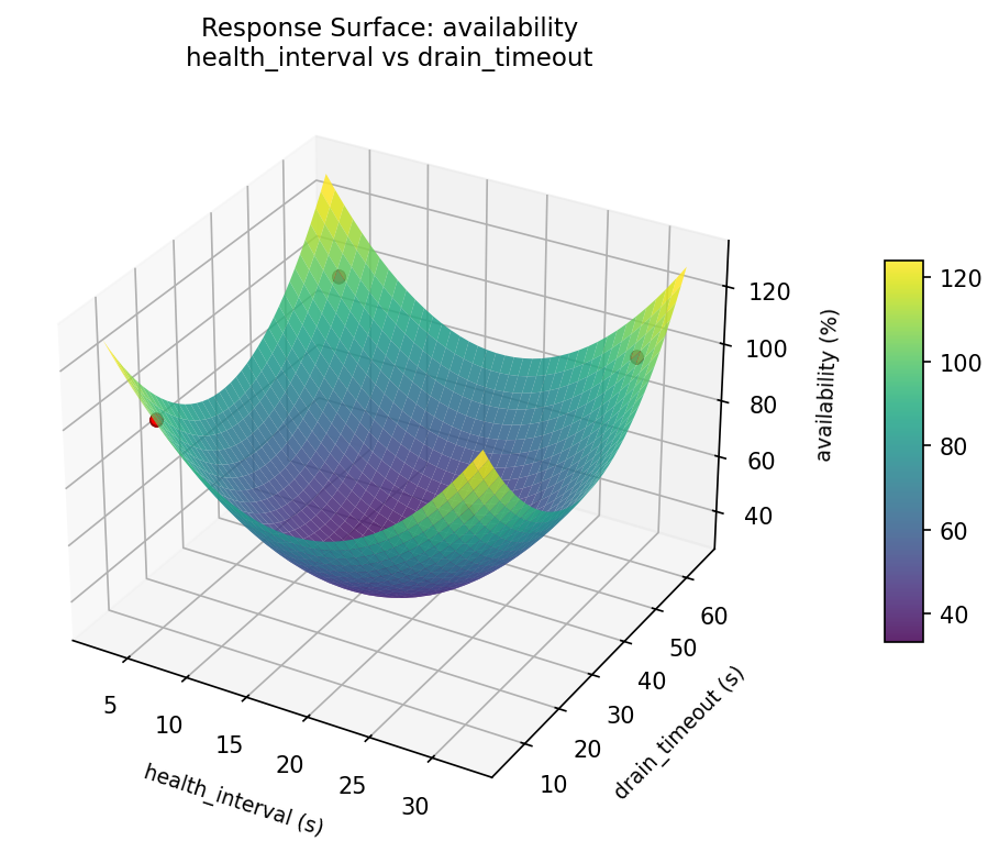
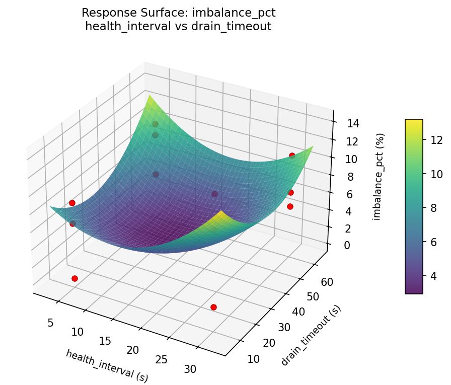
Response Surface Plots
3D surfaces fitted with quadratic RSM. Red dots are observed data points.
availability health interval vs drain timeout
imbalance pct health interval vs drain timeout
Multi-Objective Optimization
When responses compete, Derringer–Suich desirability finds the best compromise.
Each response is scaled to a 0–1 desirability, then combined via a weighted geometric mean.
Overall Desirability
D = 0.9063
Per-Response Desirability
| Response | Weight | Desirability | Predicted | Dir |
|---|
availability |
1.5 |
|
99.96 0.9545 99.96 % |
↑ |
imbalance_pct |
1.0 |
|
1.90 0.8385 1.90 % |
↓ |
Recommended Settings
| Factor | Value |
|---|
algorithm | least_conn |
health_interval | 5 s |
drain_timeout | 10 s |
Source: from observed run #2
Trade-off Summary
Sacrifice = how much worse than single-objective best.
| Response | Predicted | Best Observed | Sacrifice |
|---|
imbalance_pct | 1.90 | 0.10 | +1.80 |
Top 3 Runs by Desirability
| Run | D | Factor Settings |
|---|
| #9 | 0.8806 | algorithm=round_robin, health_interval=5, drain_timeout=10 |
| #11 | 0.7356 | algorithm=round_robin, health_interval=5, drain_timeout=60 |
Model Quality
| Response | R² | Type |
|---|
imbalance_pct | 0.2969 | linear |
Full Multi-Objective Output
============================================================
MULTI-OBJECTIVE OPTIMIZATION
Method: Derringer-Suich Desirability Function
============================================================
Overall desirability: D = 0.9063
Response Weight Desirability Predicted Direction
---------------------------------------------------------------------
availability 1.5 0.9545 99.96 % ↑
imbalance_pct 1.0 0.8385 1.90 % ↓
Recommended settings:
algorithm = least_conn
health_interval = 5 s
drain_timeout = 10 s
(from observed run #2)
Trade-off summary:
availability: 99.96 (best observed: 99.96, sacrifice: +0.00)
imbalance_pct: 1.90 (best observed: 0.10, sacrifice: +1.80)
Model quality:
availability: R² = 0.2471 (linear)
imbalance_pct: R² = 0.2969 (linear)
Top 3 observed runs by overall desirability:
1. Run #2 (D=0.9063): algorithm=least_conn, health_interval=5, drain_timeout=10
2. Run #9 (D=0.8806): algorithm=round_robin, health_interval=5, drain_timeout=10
3. Run #11 (D=0.7356): algorithm=round_robin, health_interval=5, drain_timeout=60
Full Analysis Output
=== Main Effects: availability ===
Factor Effect Std Error % Contribution
--------------------------------------------------------------
algorithm 0.2293 0.0770 58.7%
health_interval -0.0830 0.0770 21.3%
drain_timeout -0.0783 0.0770 20.1%
=== ANOVA Table: availability ===
Source DF SS MS F p-value
-----------------------------------------------------------------------------
algorithm 2 0.1273 0.0636 0.619 0.5695
health_interval 1 0.0207 0.0207 0.201 0.6695
drain_timeout 1 0.0184 0.0184 0.179 0.6868
health_interval*drain_timeout 1 0.0005 0.0005 0.005 0.9463
Error 6 0.6164 0.1027
Total 11 0.7832 0.0712
=== Interaction Effects: availability ===
Factor A Factor B Interaction % Contribution
------------------------------------------------------------------------
health_interval drain_timeout 0.0130 100.0%
=== Summary Statistics: availability ===
algorithm:
Level N Mean Std Min Max
------------------------------------------------------------
ip_hash 4 99.3995 0.2288 99.0850 99.5980
least_conn 4 99.6052 0.2587 99.2990 99.8470
round_robin 4 99.6287 0.3152 99.2410 99.9630
health_interval:
Level N Mean Std Min Max
------------------------------------------------------------
30 6 99.5860 0.3425 99.0850 99.9630
5 6 99.5030 0.1876 99.2410 99.7900
drain_timeout:
Level N Mean Std Min Max
------------------------------------------------------------
10 6 99.5837 0.3084 99.0850 99.9630
60 6 99.5053 0.2406 99.2410 99.7900
=== Main Effects: imbalance_pct ===
Factor Effect Std Error % Contribution
--------------------------------------------------------------
algorithm 3.3500 1.1645 50.1%
health_interval 2.1500 1.1645 32.2%
drain_timeout 1.1833 1.1645 17.7%
=== ANOVA Table: imbalance_pct ===
Source DF SS MS F p-value
-----------------------------------------------------------------------------
algorithm 2 26.9517 13.4758 0.606 0.5757
health_interval 1 13.8675 13.8675 0.624 0.4597
drain_timeout 1 4.2008 4.2008 0.189 0.6790
health_interval*drain_timeout 1 0.6075 0.6075 0.027 0.8741
Error 6 133.3617 22.2269
Total 11 178.9892 16.2717
=== Interaction Effects: imbalance_pct ===
Factor A Factor B Interaction % Contribution
------------------------------------------------------------------------
health_interval drain_timeout -0.4500 100.0%
=== Summary Statistics: imbalance_pct ===
algorithm:
Level N Mean Std Min Max
------------------------------------------------------------
ip_hash 4 9.4000 3.6914 6.4000 14.2000
least_conn 4 6.0500 4.5406 0.1000 10.2000
round_robin 4 6.4250 4.0541 1.9000 10.8000
health_interval:
Level N Mean Std Min Max
------------------------------------------------------------
30 6 6.2167 5.2814 0.1000 14.2000
5 6 8.3667 2.2651 5.0000 10.8000
drain_timeout:
Level N Mean Std Min Max
------------------------------------------------------------
10 6 6.7000 5.1338 0.1000 14.2000
60 6 7.8833 2.9329 4.3000 10.8000
Optimization Recommendations
=== Optimization: availability ===
Direction: maximize
Best observed run: #2
algorithm = least_conn
health_interval = 5
drain_timeout = 10
Value: 99.963
RSM Model (linear, R² = 0.3423, Adj R² = 0.0956):
Coefficients:
intercept +99.5445
algorithm +0.1460
health_interval -0.0053
drain_timeout -0.0900
RSM Model (quadratic, R² = 0.7731, Adj R² = -0.2480):
Coefficients:
intercept +33.2433
algorithm +0.1460
health_interval -0.0053
drain_timeout -0.0900
algorithm*health_interval +0.1055
algorithm*drain_timeout -0.0260
health_interval*drain_timeout +0.0552
algorithm^2 -0.2782
health_interval^2 +33.2433
drain_timeout^2 +33.2433
Curvature analysis:
health_interval coef=+33.2433 convex (has a minimum)
drain_timeout coef=+33.2433 convex (has a minimum)
algorithm coef=-0.2782 concave (has a maximum)
Predicted optimum (from linear model, at observed points):
algorithm = round_robin
health_interval = 5
drain_timeout = 10
Predicted value: 99.7858
Surface optimum (via L-BFGS-B, linear model):
algorithm = least_conn
health_interval = 5
drain_timeout = 10
Predicted value: 99.7858
Model quality: Weak fit — consider adding center points or using a different design.
Factor importance:
1. algorithm (effect: 0.4, contribution: 69.0%)
2. drain_timeout (effect: -0.2, contribution: 29.3%)
3. health_interval (effect: 0.0, contribution: 1.7%)
=== Optimization: imbalance_pct ===
Direction: minimize
Best observed run: #9
algorithm = round_robin
health_interval = 30
drain_timeout = 10
Value: 0.1
RSM Model (linear, R² = 0.3128, Adj R² = 0.0550):
Coefficients:
intercept +7.2917
algorithm -2.1625
health_interval -0.0750
drain_timeout +1.2417
RSM Model (quadratic, R² = 0.6254, Adj R² = -1.0602):
Coefficients:
intercept +1.8000
algorithm -2.1625
health_interval -0.0750
drain_timeout +1.2417
algorithm*health_interval -1.8375
algorithm*drain_timeout +0.7875
health_interval*drain_timeout -0.4583
algorithm^2 +2.8375
health_interval^2 +1.8000
drain_timeout^2 +1.8000
Curvature analysis:
algorithm coef=+2.8375 convex (has a minimum)
drain_timeout coef=+1.8000 convex (has a minimum)
health_interval coef=+1.8000 convex (has a minimum)
Notable interactions:
algorithm*health_interval coef=-1.8375 (antagonistic)
algorithm*drain_timeout coef=+0.7875 (synergistic)
health_interval*drain_timeout coef=-0.4583 (antagonistic)
Predicted optimum (from linear model, at observed points):
algorithm = ip_hash
health_interval = 5
drain_timeout = 60
Predicted value: 10.7708
Surface optimum (via L-BFGS-B, linear model):
algorithm = least_conn
health_interval = 30
drain_timeout = 10
Predicted value: 3.8125
Model quality: Weak fit — consider adding center points or using a different design.
Factor importance:
1. algorithm (effect: 5.0, contribution: 65.5%)
2. drain_timeout (effect: 2.5, contribution: 32.5%)
3. health_interval (effect: 0.2, contribution: 2.0%)