Summary
This experiment investigates database connection pooling. Box-Behnken design to optimize connection pool size, idle timeout, and max lifetime for throughput.
The design varies 3 factors: pool size (conns), ranging from 5 to 50, idle timeout (s), ranging from 30 to 300, and max lifetime (s), ranging from 300 to 3600. The goal is to optimize 2 responses: throughput qps (qps) (maximize) and p95 latency ms (ms) (minimize). Fixed conditions held constant across all runs include db engine = postgresql, ssl = true.
A Box-Behnken design was chosen because it efficiently fits quadratic models with 3 continuous factors while avoiding extreme corner combinations — requiring only 15 runs instead of the 8 needed for a full factorial at two levels.
Quadratic response surface models were fitted to capture potential curvature and factor interactions. The RSM contour plots below visualize how pairs of factors jointly affect each response.
Key Findings
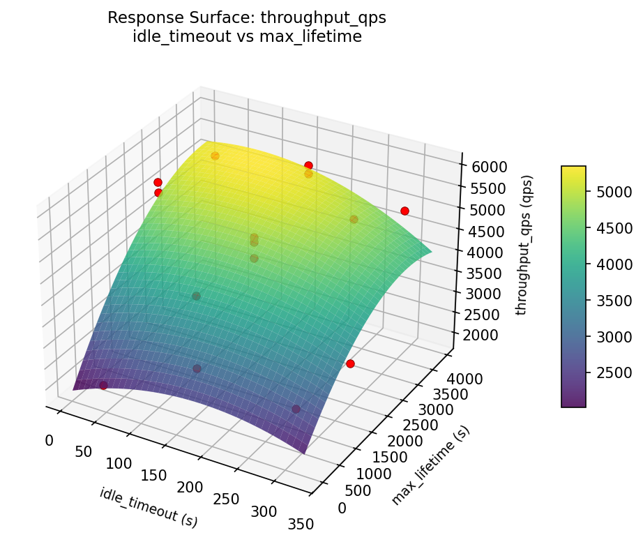
For throughput qps, the most influential factors were idle timeout (67.4%), max lifetime (17.5%), pool size (15.1%). The best observed value was 5964.0 (at pool size = 50, idle timeout = 300, max lifetime = 1950).
For p95 latency ms, the most influential factors were idle timeout (64.2%), max lifetime (21.4%), pool size (14.3%). The best observed value was 9.3 (at pool size = 27.5, idle timeout = 30, max lifetime = 3600).
Recommended Next Steps
- Run confirmation experiments at the predicted optimal settings to validate the model.
- Consider whether any fixed factors should be varied in a future study.
Experimental Setup
Factors
| Factor | Low | High | Unit |
|---|
pool_size | 5 | 50 | conns |
idle_timeout | 30 | 300 | s |
max_lifetime | 300 | 3600 | s |
Fixed: db_engine = postgresql, ssl = true
Responses
| Response | Direction | Unit |
|---|
throughput_qps | ↑ maximize | qps |
p95_latency_ms | ↓ minimize | ms |
Configuration
{
"metadata": {
"name": "Database Connection Pooling",
"description": "Box-Behnken design to optimize connection pool size, idle timeout, and max lifetime for throughput"
},
"factors": [
{
"name": "pool_size",
"levels": [
"5",
"50"
],
"type": "continuous",
"unit": "conns"
},
{
"name": "idle_timeout",
"levels": [
"30",
"300"
],
"type": "continuous",
"unit": "s"
},
{
"name": "max_lifetime",
"levels": [
"300",
"3600"
],
"type": "continuous",
"unit": "s"
}
],
"fixed_factors": {
"db_engine": "postgresql",
"ssl": "true"
},
"responses": [
{
"name": "throughput_qps",
"optimize": "maximize",
"unit": "qps"
},
{
"name": "p95_latency_ms",
"optimize": "minimize",
"unit": "ms"
}
],
"settings": {
"operation": "box_behnken",
"test_script": "use_cases/31_database_connection_pooling/sim.sh"
}
}
Experimental Matrix
The Box-Behnken Design produces 15 runs. Each row is one experiment with specific factor settings.
| Run | pool_size | idle_timeout | max_lifetime |
|---|
| 1 | 27.5 | 30 | 300 |
| 2 | 27.5 | 165 | 1950 |
| 3 | 50 | 165 | 3600 |
| 4 | 50 | 165 | 300 |
| 5 | 27.5 | 165 | 1950 |
| 6 | 27.5 | 165 | 1950 |
| 7 | 5 | 165 | 3600 |
| 8 | 50 | 30 | 1950 |
| 9 | 27.5 | 30 | 3600 |
| 10 | 50 | 300 | 1950 |
| 11 | 5 | 165 | 300 |
| 12 | 27.5 | 300 | 3600 |
| 13 | 5 | 30 | 1950 |
| 14 | 5 | 300 | 1950 |
| 15 | 27.5 | 300 | 300 |
Step-by-Step Workflow
1
Preview the design
$ doe info --config use_cases/31_database_connection_pooling/config.json
2
Generate the runner script
$ doe generate --config use_cases/31_database_connection_pooling/config.json \
--output use_cases/31_database_connection_pooling/results/run.sh --seed 42
3
Execute the experiments
$ bash use_cases/31_database_connection_pooling/results/run.sh
4
Analyze results
$ doe analyze --config use_cases/31_database_connection_pooling/config.json
5
Get optimization recommendations
$ doe optimize --config use_cases/31_database_connection_pooling/config.json
6
Multi-objective optimization
With 2 competing responses, use --multi to find the best compromise via Derringer–Suich desirability.
$ doe optimize --config use_cases/31_database_connection_pooling/config.json --multi
7
Generate the HTML report
$ doe report --config use_cases/31_database_connection_pooling/config.json \
--output use_cases/31_database_connection_pooling/results/report.html
Features Exercised
| Feature | Value |
|---|
| Design type | box_behnken |
| Factor types | continuous (all 3) |
| Arg style | double-dash |
| Responses | 2 (throughput_qps ↑, p95_latency_ms ↓) |
| Total runs | 15 |
Analysis Results
Generated from actual experiment runs using the DOE Helper Tool.
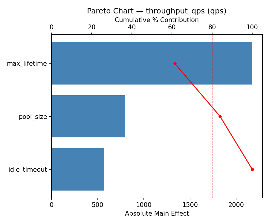
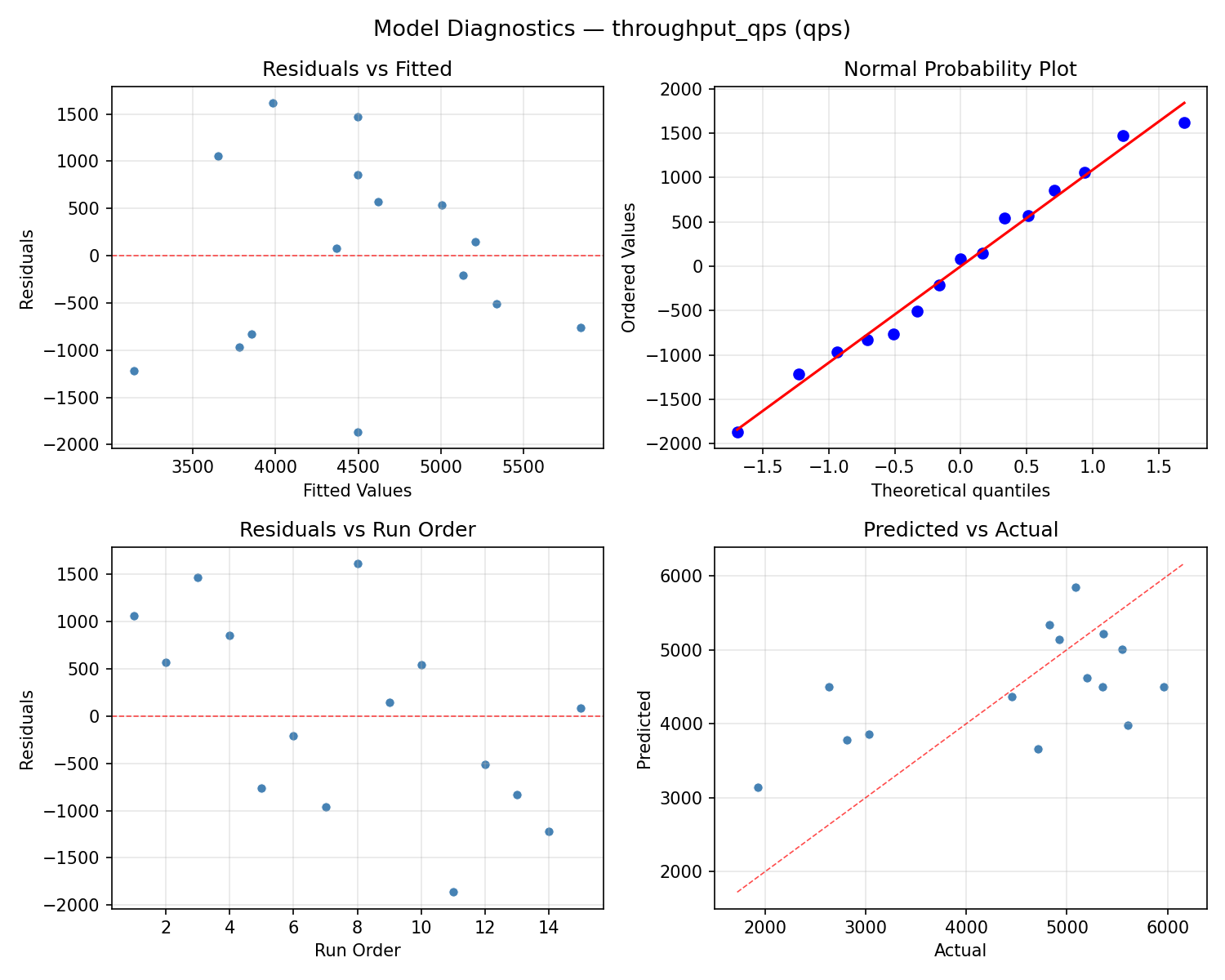
Response: throughput_qps
Top factors: idle_timeout (67.4%), max_lifetime (17.5%), pool_size (15.1%).
ANOVA
| Source | DF | SS | MS | F | p-value |
|---|
| Source | DF | SS | MS | F | p-value |
| pool_size | 2 | 729970.1833 | 364985.0917 | 0.188 | 0.8320 |
| idle_timeout | 2 | 10819680.3262 | 5409840.1631 | 2.789 | 0.1205 |
| max_lifetime | 2 | 778742.2190 | 389371.1095 | 0.201 | 0.8221 |
| Lack | of | Fit | 6 | 5981098.2048 | 996849.7008 |
| Pure | Error | 2 | 3879386.0000 | | |
| Error | 8 | 9860484.2048 | 1939693.0000 | | |
| Total | 14 | 22188876.9333 | 1584919.7810 | | |
Pareto Chart
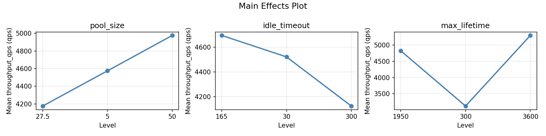
Main Effects Plot
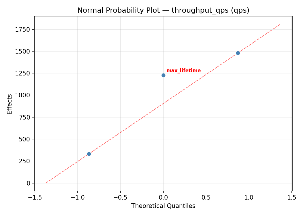
Normal Probability Plot of Effects
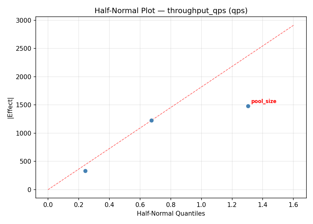
Half-Normal Plot of Effects
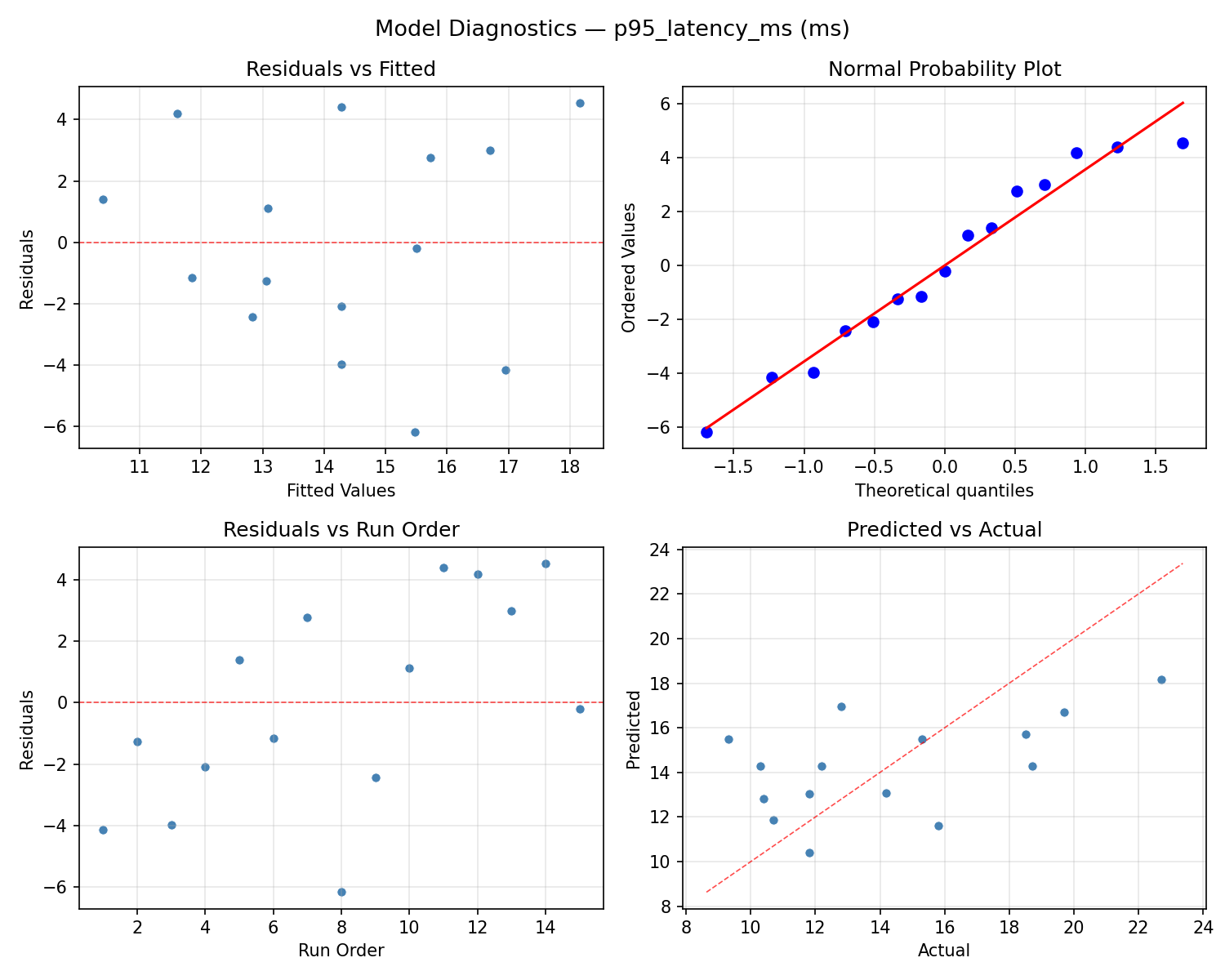
Model Diagnostics
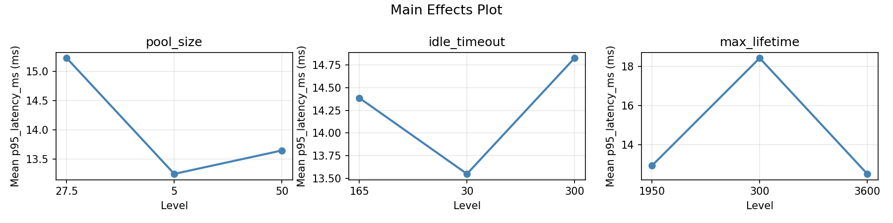
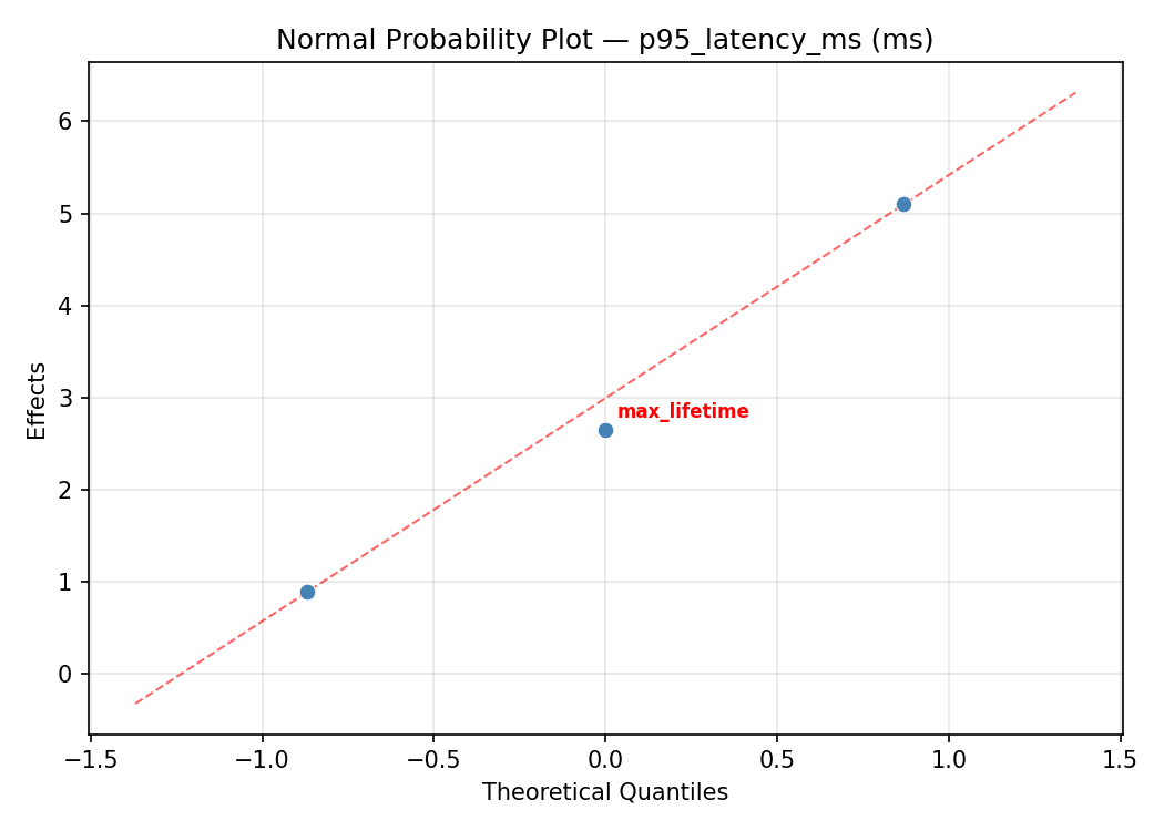
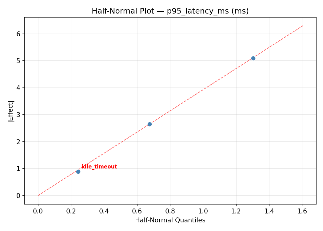
Response: p95_latency_ms
Top factors: idle_timeout (64.2%), max_lifetime (21.4%), pool_size (14.3%).
ANOVA
| Source | DF | SS | MS | F | p-value |
|---|
| Source | DF | SS | MS | F | p-value |
| pool_size | 2 | 8.2522 | 4.1261 | 0.292 | 0.7543 |
| idle_timeout | 2 | 133.5879 | 66.7940 | 4.729 | 0.0441 |
| max_lifetime | 2 | 13.6404 | 6.8202 | 0.483 | 0.6339 |
| Lack | of | Fit | 6 | 44.5768 | 7.4295 |
| Pure | Error | 2 | 28.2467 | | |
| Error | 8 | 72.8234 | 14.1233 | | |
| Total | 14 | 228.3040 | 16.3074 | | |
Pareto Chart

Main Effects Plot
Normal Probability Plot of Effects
Half-Normal Plot of Effects
Model Diagnostics
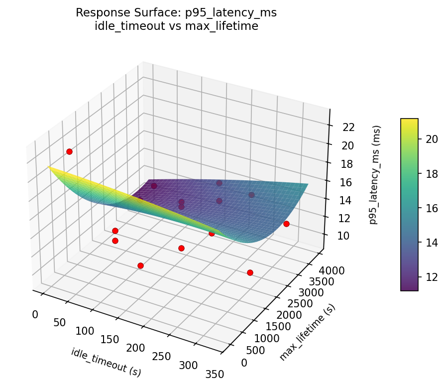
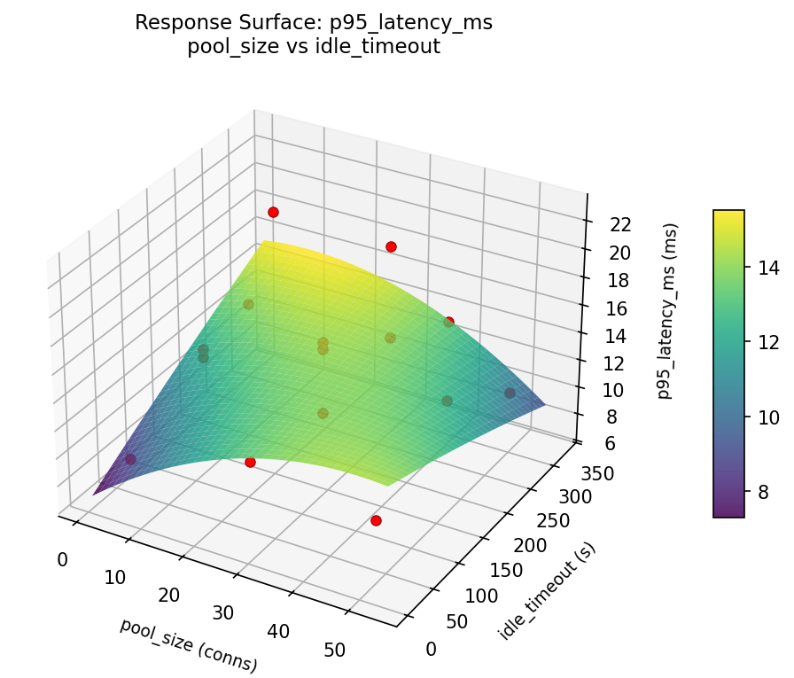
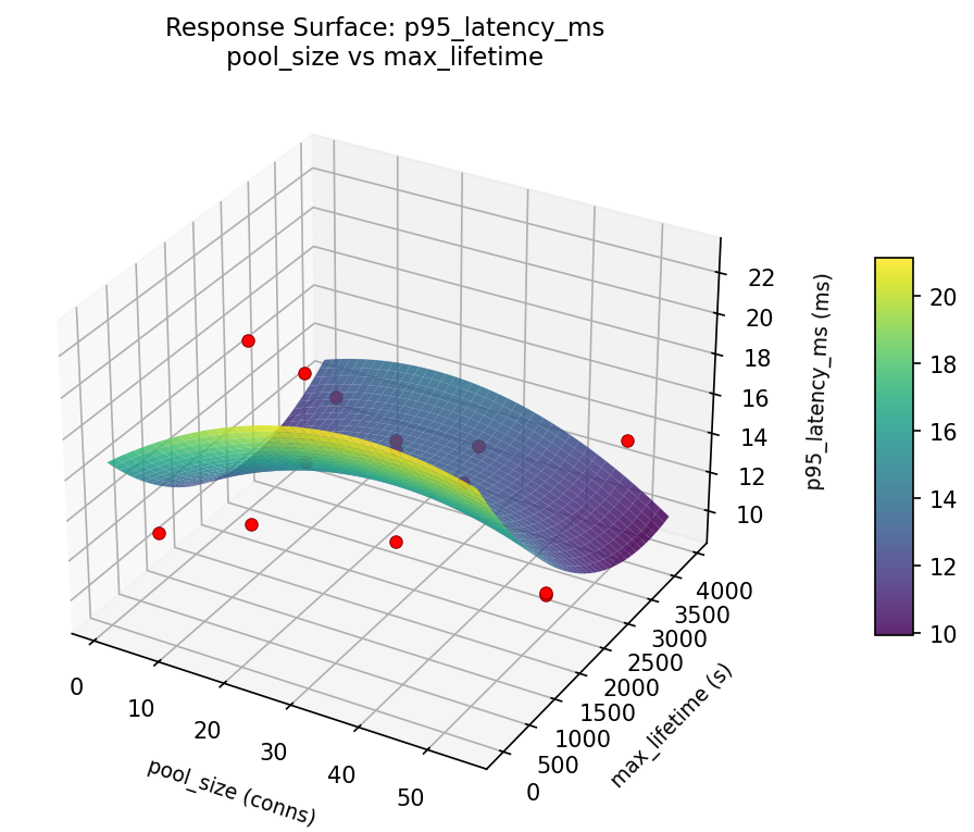
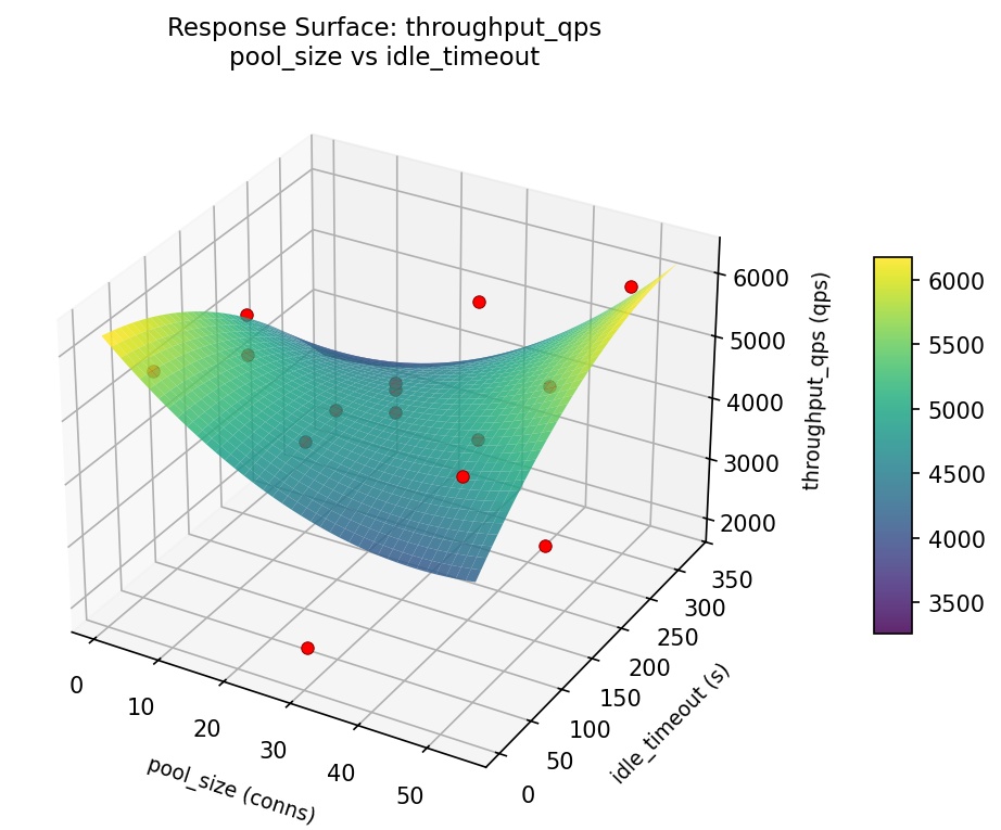
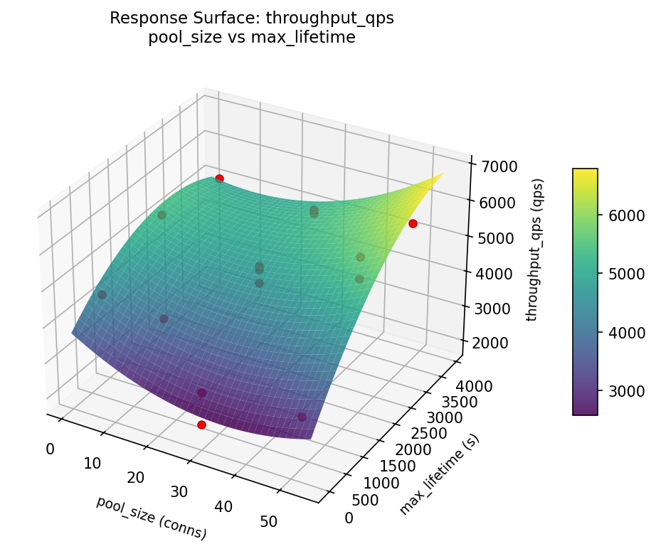
Response Surface Plots
3D surfaces fitted with quadratic RSM. Red dots are observed data points.
p95 latency ms idle timeout vs max lifetime
p95 latency ms pool size vs idle timeout
p95 latency ms pool size vs max lifetime
throughput qps idle timeout vs max lifetime
throughput qps pool size vs idle timeout
throughput qps pool size vs max lifetime
Multi-Objective Optimization
When responses compete, Derringer–Suich desirability finds the best compromise.
Each response is scaled to a 0–1 desirability, then combined via a weighted geometric mean.
Overall Desirability
D = 0.9268
Per-Response Desirability
| Response | Weight | Desirability | Predicted | Dir |
|---|
throughput_qps |
1.5 |
|
5964.00 0.9545 5964.00 qps |
↑ |
p95_latency_ms |
1.0 |
|
10.30 0.8867 10.30 ms |
↓ |
Recommended Settings
| Factor | Value |
|---|
pool_size | 27.5 conns |
idle_timeout | 30 s |
max_lifetime | 3600 s |
Source: from observed run #3
Trade-off Summary
Sacrifice = how much worse than single-objective best.
| Response | Predicted | Best Observed | Sacrifice |
|---|
p95_latency_ms | 10.30 | 9.30 | +1.00 |
Top 3 Runs by Desirability
| Run | D | Factor Settings |
|---|
| #8 | 0.9048 | pool_size=27.5, idle_timeout=300, max_lifetime=300 |
| #9 | 0.8423 | pool_size=50, idle_timeout=30, max_lifetime=1950 |
Model Quality
| Response | R² | Type |
|---|
p95_latency_ms | 0.6584 | quadratic |
Full Multi-Objective Output
============================================================
MULTI-OBJECTIVE OPTIMIZATION
Method: Derringer-Suich Desirability Function
============================================================
Overall desirability: D = 0.9268
Response Weight Desirability Predicted Direction
---------------------------------------------------------------------
throughput_qps 1.5 0.9545 5964.00 qps ↑
p95_latency_ms 1.0 0.8867 10.30 ms ↓
Recommended settings:
pool_size = 27.5 conns
idle_timeout = 30 s
max_lifetime = 3600 s
(from observed run #3)
Trade-off summary:
throughput_qps: 5964.00 (best observed: 5964.00, sacrifice: +0.00)
p95_latency_ms: 10.30 (best observed: 9.30, sacrifice: +1.00)
Model quality:
throughput_qps: R² = 0.1691 (linear)
p95_latency_ms: R² = 0.6584 (quadratic)
Top 3 observed runs by overall desirability:
1. Run #3 (D=0.9268): pool_size=27.5, idle_timeout=30, max_lifetime=3600
2. Run #8 (D=0.9048): pool_size=27.5, idle_timeout=300, max_lifetime=300
3. Run #9 (D=0.8423): pool_size=50, idle_timeout=30, max_lifetime=1950
Full Analysis Output
=== Main Effects: throughput_qps ===
Factor Effect Std Error % Contribution
--------------------------------------------------------------
idle_timeout 2100.2500 325.0559 67.4%
max_lifetime 545.4286 325.0559 17.5%
pool_size 469.2500 325.0559 15.1%
=== ANOVA Table: throughput_qps ===
Source DF SS MS F p-value
-----------------------------------------------------------------------------
pool_size 2 729970.1833 364985.0917 0.188 0.8320
idle_timeout 2 10819680.3262 5409840.1631 2.789 0.1205
max_lifetime 2 778742.2190 389371.1095 0.201 0.8221
Lack of Fit 6 5981098.2048 996849.7008 0.514 0.7768
Pure Error 2 3879386.0000 1939693.0000
Error 8 9860484.2048 1939693.0000
Total 14 22188876.9333 1584919.7810
=== Summary Statistics: throughput_qps ===
pool_size:
Level N Mean Std Min Max
------------------------------------------------------------
27.5 7 4261.0000 1352.9703 2632.0000 5549.0000
5 4 4672.0000 1857.3508 1926.0000 5964.0000
50 4 4730.2500 205.3280 4451.0000 4927.0000
idle_timeout:
Level N Mean Std Min Max
------------------------------------------------------------
165 7 4885.8571 1032.7390 2818.0000 5964.0000
30 4 5204.5000 356.8029 4715.0000 5549.0000
300 4 3104.2500 1236.6585 1926.0000 4828.0000
max_lifetime:
Level N Mean Std Min Max
------------------------------------------------------------
1950 7 4274.5714 1342.0782 1926.0000 5351.0000
300 4 4820.0000 1266.2477 3031.0000 5964.0000
3600 4 4558.5000 1389.5972 2632.0000 5602.0000
=== Main Effects: p95_latency_ms ===
Factor Effect Std Error % Contribution
--------------------------------------------------------------
idle_timeout 6.9250 1.0427 64.2%
max_lifetime 2.3107 1.0427 21.4%
pool_size 1.5464 1.0427 14.3%
=== ANOVA Table: p95_latency_ms ===
Source DF SS MS F p-value
-----------------------------------------------------------------------------
pool_size 2 8.2522 4.1261 0.292 0.7543
idle_timeout 2 133.5879 66.7940 4.729 0.0441
max_lifetime 2 13.6404 6.8202 0.483 0.6339
Lack of Fit 6 44.5768 7.4295 0.526 0.7706
Pure Error 2 28.2467 14.1233
Error 8 72.8234 14.1233
Total 14 228.3040 16.3074
=== Summary Statistics: p95_latency_ms ===
pool_size:
Level N Mean Std Min Max
------------------------------------------------------------
27.5 7 15.0714 3.8270 10.4000 19.7000
5 4 13.5250 6.2024 9.3000 22.7000
50 4 13.6500 2.3643 10.7000 15.8000
idle_timeout:
Level N Mean Std Min Max
------------------------------------------------------------
165 7 12.5857 3.2324 9.3000 18.5000
30 4 12.3000 1.6042 10.4000 14.2000
300 4 19.2250 2.8465 15.8000 22.7000
max_lifetime:
Level N Mean Std Min Max
------------------------------------------------------------
1950 7 15.0857 4.1890 11.8000 22.7000
300 4 12.7750 4.6198 10.3000 19.7000
3600 4 14.3750 3.8879 9.3000 18.7000
Optimization Recommendations
=== Optimization: throughput_qps ===
Direction: maximize
Best observed run: #3
pool_size = 50
idle_timeout = 300
max_lifetime = 1950
Value: 5964.0
RSM Model (linear, R² = 0.2952, Adj R² = 0.1030):
Coefficients:
intercept +4495.7333
pool_size -269.0000
idle_timeout +806.0000
max_lifetime -311.0000
RSM Model (quadratic, R² = 0.5618, Adj R² = -0.2270):
Coefficients:
intercept +4065.3333
pool_size -269.0000
idle_timeout +806.0000
max_lifetime -311.0000
pool_size*idle_timeout +328.0000
pool_size*max_lifetime -329.0000
idle_timeout*max_lifetime -178.0000
pool_size^2 -525.1667
idle_timeout^2 +429.8333
max_lifetime^2 +902.3333
Curvature analysis:
max_lifetime coef=+902.3333 convex (has a minimum)
pool_size coef=-525.1667 concave (has a maximum)
idle_timeout coef=+429.8333 convex (has a minimum)
Notable interactions:
pool_size*max_lifetime coef=-329.0000 (antagonistic)
pool_size*idle_timeout coef=+328.0000 (synergistic)
idle_timeout*max_lifetime coef=-178.0000 (antagonistic)
Predicted optimum (from linear model, at observed points):
pool_size = 27.5
idle_timeout = 300
max_lifetime = 300
Predicted value: 5612.7333
Surface optimum (via L-BFGS-B, linear model):
pool_size = 5
idle_timeout = 300
max_lifetime = 300
Predicted value: 5881.7333
Model quality: Weak fit — consider adding center points or using a different design.
Factor importance:
1. idle_timeout (effect: 1612.0, contribution: 43.3%)
2. max_lifetime (effect: 1220.1, contribution: 32.8%)
3. pool_size (effect: 889.3, contribution: 23.9%)
=== Optimization: p95_latency_ms ===
Direction: minimize
Best observed run: #8
pool_size = 27.5
idle_timeout = 30
max_lifetime = 3600
Value: 9.3
RSM Model (linear, R² = 0.2637, Adj R² = 0.0629):
Coefficients:
intercept +14.2800
pool_size +1.8500
idle_timeout -2.0250
max_lifetime -0.0500
RSM Model (quadratic, R² = 0.4338, Adj R² = -0.5852):
Coefficients:
intercept +14.8333
pool_size +1.8500
idle_timeout -2.0250
max_lifetime -0.0500
pool_size*idle_timeout -1.0250
pool_size*max_lifetime +0.7250
idle_timeout*max_lifetime +0.1250
pool_size^2 +1.9208
idle_timeout^2 -1.2292
max_lifetime^2 -1.7292
Curvature analysis:
pool_size coef=+1.9208 convex (has a minimum)
max_lifetime coef=-1.7292 concave (has a maximum)
idle_timeout coef=-1.2292 concave (has a maximum)
Notable interactions:
pool_size*idle_timeout coef=-1.0250 (antagonistic)
pool_size*max_lifetime coef=+0.7250 (synergistic)
Predicted optimum (from linear model, at observed points):
pool_size = 50
idle_timeout = 30
max_lifetime = 1950
Predicted value: 18.1550
Surface optimum (via L-BFGS-B, linear model):
pool_size = 5
idle_timeout = 300
max_lifetime = 3600
Predicted value: 10.3550
Model quality: Weak fit — consider adding center points or using a different design.
Factor importance:
1. idle_timeout (effect: 4.0, contribution: 41.1%)
2. pool_size (effect: 4.0, contribution: 40.4%)
3. max_lifetime (effect: 1.8, contribution: 18.5%)