Vulnerability Scan Scheduling

Summary

This experiment investigates vulnerability scan scheduling. Central Composite design to optimize scan threads, port range, and timeout for scan duration and coverage.

The design varies 3 factors: scan threads (threads), ranging from 2 to 32, port range size (ports), ranging from 100 to 65535, and timeout ms (ms), ranging from 500 to 10000. The goal is to optimize 2 responses: scan duration min (min) (minimize) and coverage pct (%) (maximize). Fixed conditions held constant across all runs include scanner = openvas, target network = 10.0.0.0/16.

A Central Composite Design (CCD) was selected to fit a full quadratic response surface model, including curvature and interaction effects. With 3 factors this produces 22 runs including center points and axial (star) points that extend beyond the factorial range.

Quadratic response surface models were fitted to capture potential curvature and factor interactions. The RSM contour plots below visualize how pairs of factors jointly affect each response.

Key Findings

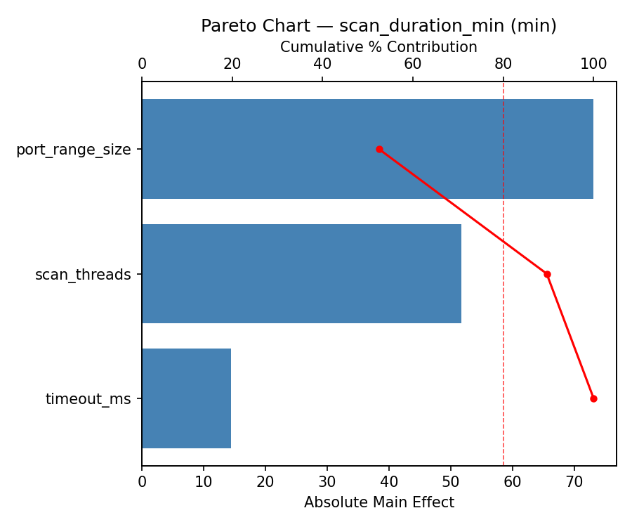
For scan duration min, the most influential factors were port range size (53.9%), timeout ms (37.4%), scan threads (8.8%). The best observed value was 14.6 (at scan threads = 17, port range size = 32817.5, timeout ms = 5250).

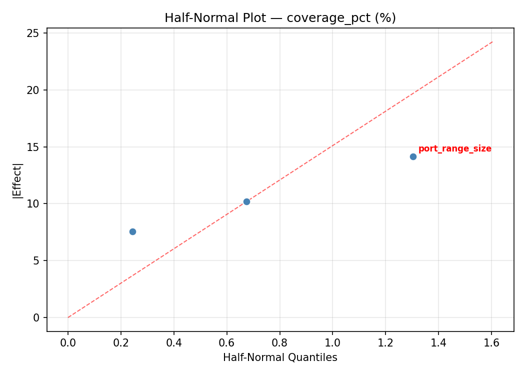
For coverage pct, the most influential factors were port range size (52.5%), timeout ms (33.4%), scan threads (14.1%). The best observed value was 91.3 (at scan threads = 17, port range size = 32817.5, timeout ms = 5250).

Recommended Next Steps

Run confirmation experiments at the predicted optimal settings to validate the model.
Consider whether any fixed factors should be varied in a future study.

Experimental Setup

Factors

Factor	Low	High	Unit
`scan_threads`	2	32	threads
`port_range_size`	100	65535	ports
`timeout_ms`	500	10000	ms

Fixed: scanner = openvas, target_network = 10.0.0.0/16

Responses

Response	Direction	Unit
`scan_duration_min`	↓ minimize	min
`coverage_pct`	↑ maximize	%

Configuration

use_cases/60_vulnerability_scan_scheduling/config.json

{
  "metadata": {
    "name": "Vulnerability Scan Scheduling",
    "description": "Central Composite design to optimize scan threads, port range, and timeout for scan duration and coverage"
  },
  "factors": [
    {
      "name": "scan_threads",
      "levels": [
        "2",
        "32"
      ],
      "type": "continuous",
      "unit": "threads"
    },
    {
      "name": "port_range_size",
      "levels": [
        "100",
        "65535"
      ],
      "type": "continuous",
      "unit": "ports"
    },
    {
      "name": "timeout_ms",
      "levels": [
        "500",
        "10000"
      ],
      "type": "continuous",
      "unit": "ms"
    }
  ],
  "fixed_factors": {
    "scanner": "openvas",
    "target_network": "10.0.0.0/16"
  },
  "responses": [
    {
      "name": "scan_duration_min",
      "optimize": "minimize",
      "unit": "min"
    },
    {
      "name": "coverage_pct",
      "optimize": "maximize",
      "unit": "%"
    }
  ],
  "settings": {
    "operation": "central_composite",
    "test_script": "use_cases/60_vulnerability_scan_scheduling/sim.sh"
  }
}

Experimental Matrix

The Central Composite Design produces 22 runs. Each row is one experiment with specific factor settings.

Run	`scan_threads`	`port_range_size`	`timeout_ms`
1	17	32817.5	5250
2	32	100	10000
3	2	65535	500
4	17	92551.2	5250
5	17	32817.5	5250
6	-10.3861	32817.5	5250
7	17	32817.5	-3422.27
8	17	32817.5	5250
9	32	65535	500
10	44.3861	32817.5	5250
11	17	32817.5	5250
12	17	-26916.2	5250
13	17	32817.5	5250
14	2	100	10000
15	17	32817.5	5250
16	32	100	500
17	17	32817.5	13922.3
18	32	65535	10000
19	17	32817.5	5250
20	2	100	500
21	2	65535	10000
22	17	32817.5	5250

Step-by-Step Workflow

1

Preview the design

Terminal

$ doe info --config use_cases/60_vulnerability_scan_scheduling/config.json

2

Generate the runner script

Terminal

$ doe generate --config use_cases/60_vulnerability_scan_scheduling/config.json \
    --output use_cases/60_vulnerability_scan_scheduling/results/run.sh --seed 42

3

Execute the experiments

Terminal

$ bash use_cases/60_vulnerability_scan_scheduling/results/run.sh

4

Analyze results

Terminal

$ doe analyze --config use_cases/60_vulnerability_scan_scheduling/config.json

5

Get optimization recommendations

Terminal

$ doe optimize --config use_cases/60_vulnerability_scan_scheduling/config.json

6

Multi-objective optimization

With 2 competing responses, use --multi to find the best compromise via Derringer–Suich desirability.

Terminal

$ doe optimize --config use_cases/60_vulnerability_scan_scheduling/config.json --multi

7

Generate the HTML report

Terminal

$ doe report --config use_cases/60_vulnerability_scan_scheduling/config.json \
    --output use_cases/60_vulnerability_scan_scheduling/results/report.html

Features Exercised

Feature	Value
Design type	`central_composite`
Factor types	`continuous` (all 3)
Arg style	`double-dash`
Responses	2 (scan_duration_min ↓, coverage_pct ↑)
Total runs	22

Analysis Results

Generated from actual experiment runs using the DOE Helper Tool.

Response: scan_duration_min

Top factors: port_range_size (53.9%), timeout_ms (37.4%), scan_threads (8.8%).

ANOVA

Source	DF	SS	MS	F	p-value
Source	DF	SS	MS	F	p-value
scan_threads	4	370.9970	92.7492	0.068	0.9901
port_range_size	4	7634.2395	1908.5599	1.400	0.3092
timeout_ms	4	5171.2970	1292.8242	0.948	0.4797
Lack	of	Fit	2	1426.4715	713.2357
Pure	Error	7	9545.3587
Error	9	10971.8302	1363.6227
Total	21	24148.3636	1149.9221

Pareto Chart

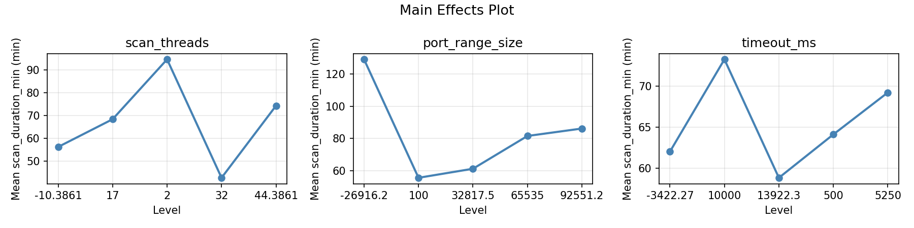
Main Effects Plot

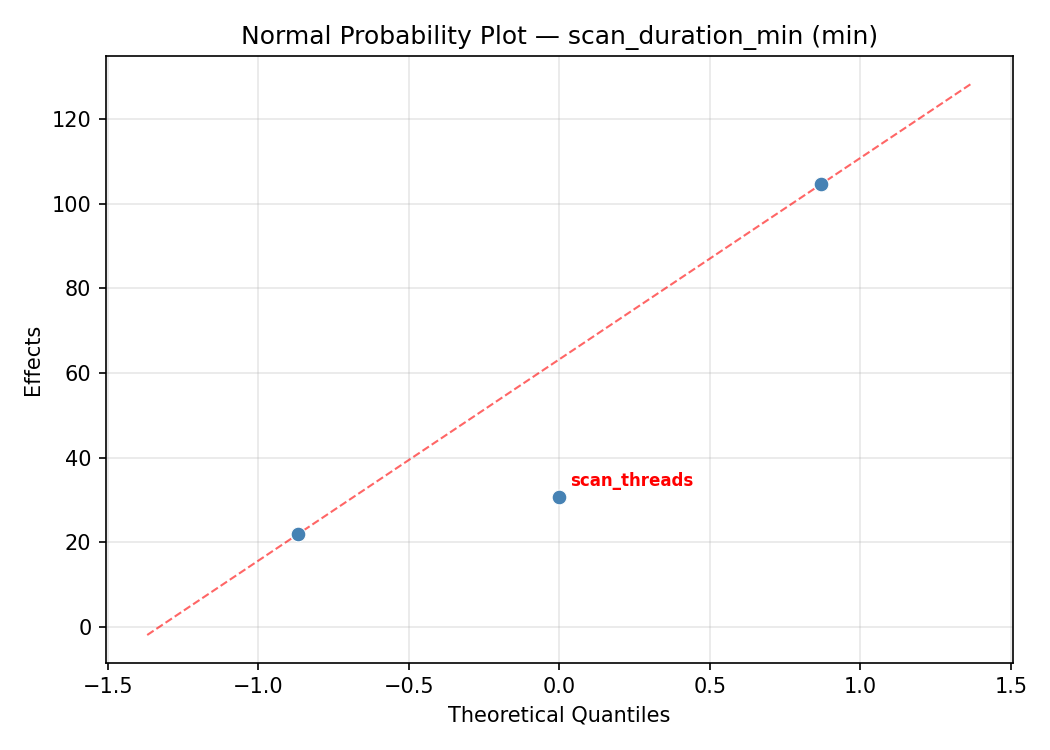
Normal Probability Plot of Effects

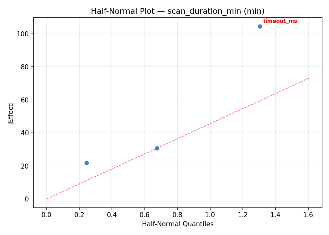
Normal probability plot for scan_duration_min

Half-Normal Plot of Effects

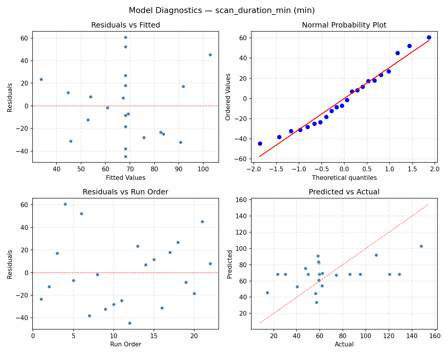
Model Diagnostics

Response: coverage_pct

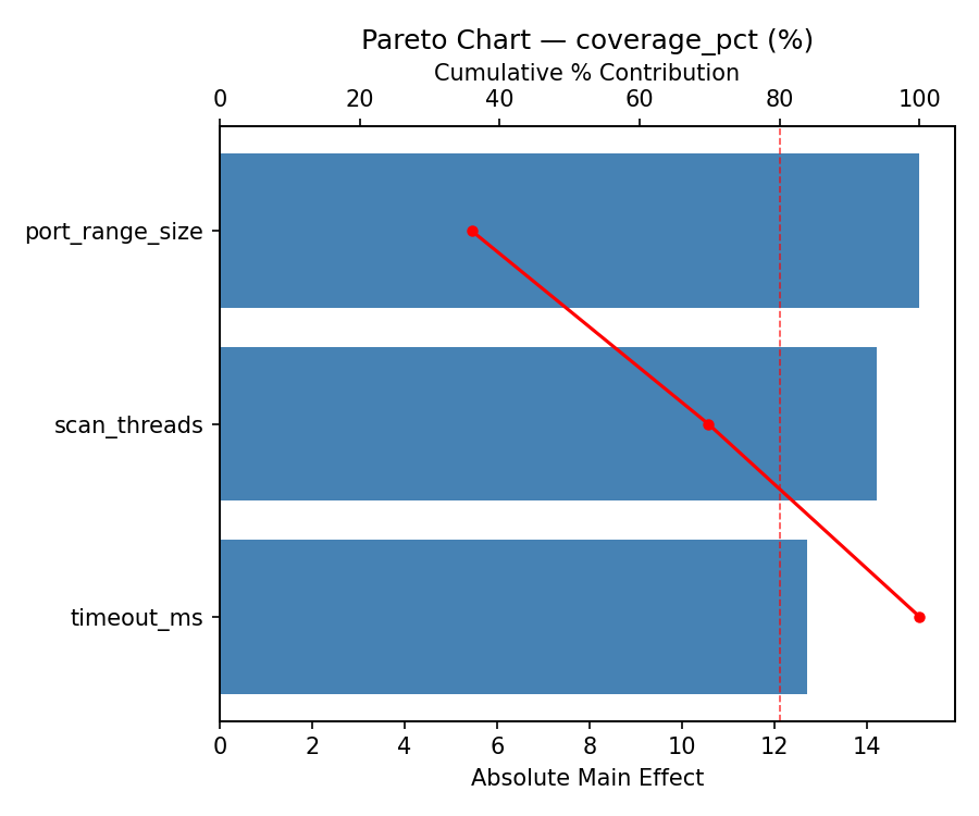
Top factors: port_range_size (52.5%), timeout_ms (33.4%), scan_threads (14.1%).

ANOVA

Source	DF	SS	MS	F	p-value
Source	DF	SS	MS	F	p-value
scan_threads	4	47.7832	11.9458	0.054	0.9936
port_range_size	4	729.8632	182.4658	0.820	0.5441
timeout_ms	4	757.3365	189.3341	0.850	0.5279
Lack	of	Fit	2	376.5216	188.2608
Pure	Error	7	1558.4688
Error	9	1934.9903	222.6384
Total	21	3469.9732	165.2368

Pareto Chart

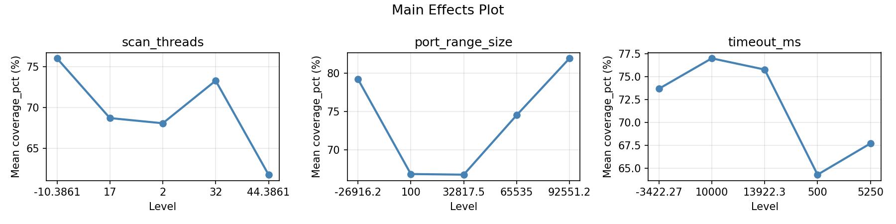
Main Effects Plot

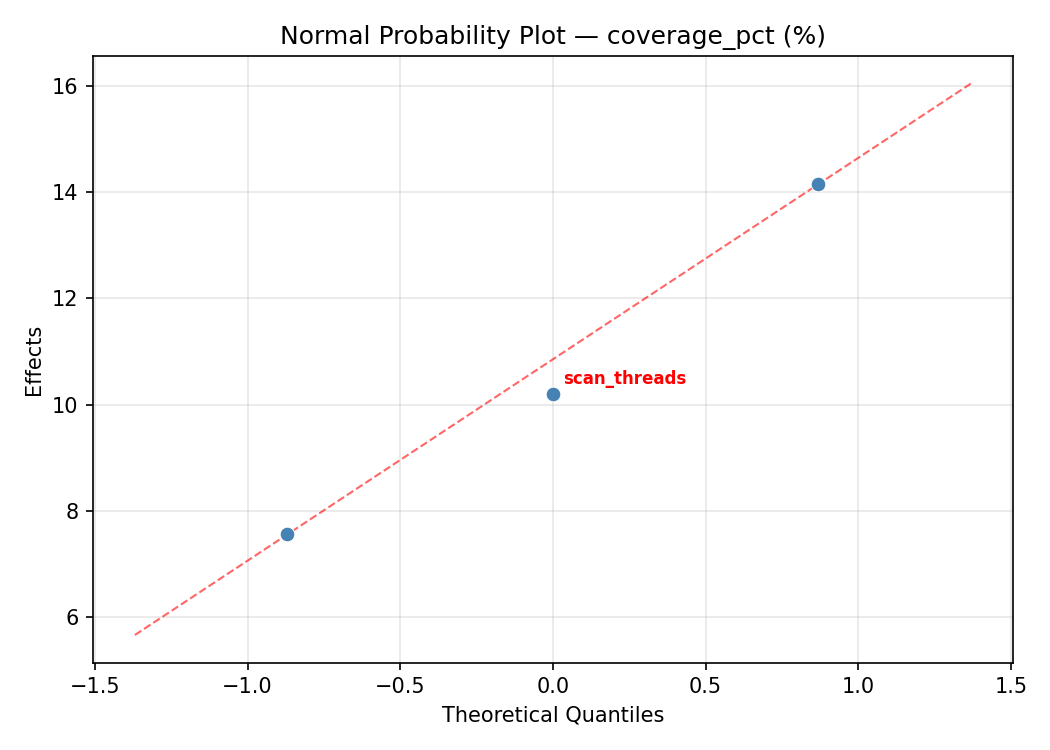
Normal Probability Plot of Effects

Normal probability plot for coverage_pct

Half-Normal Plot of Effects

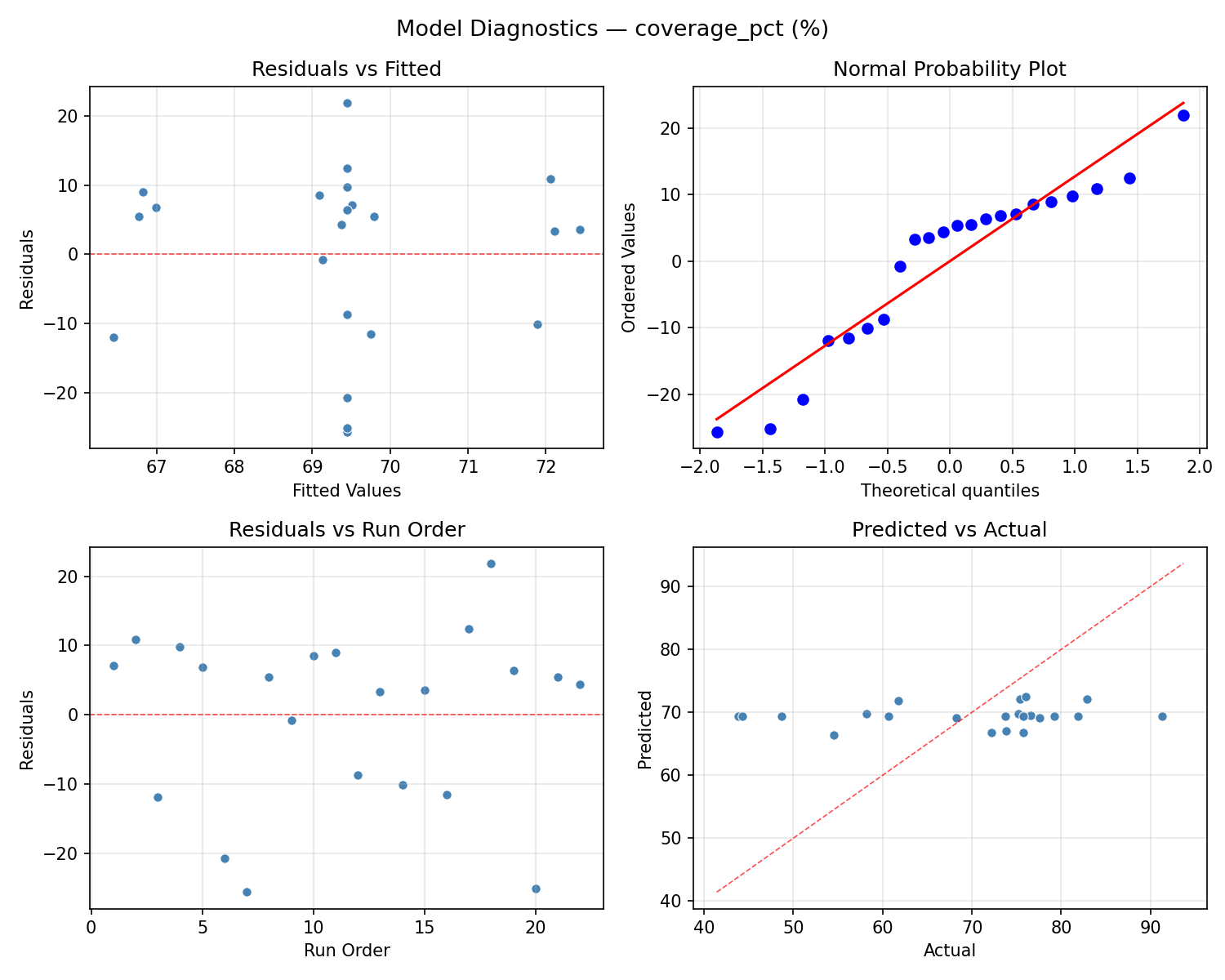
Model Diagnostics

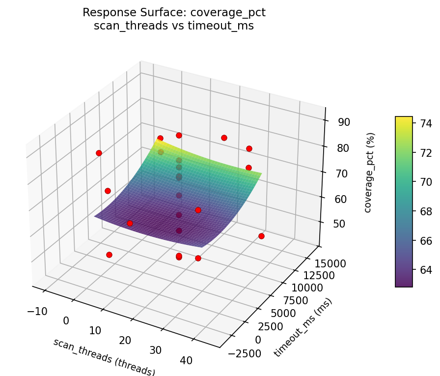
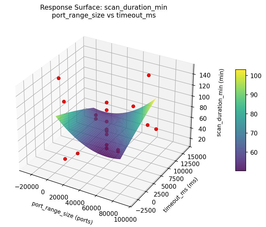
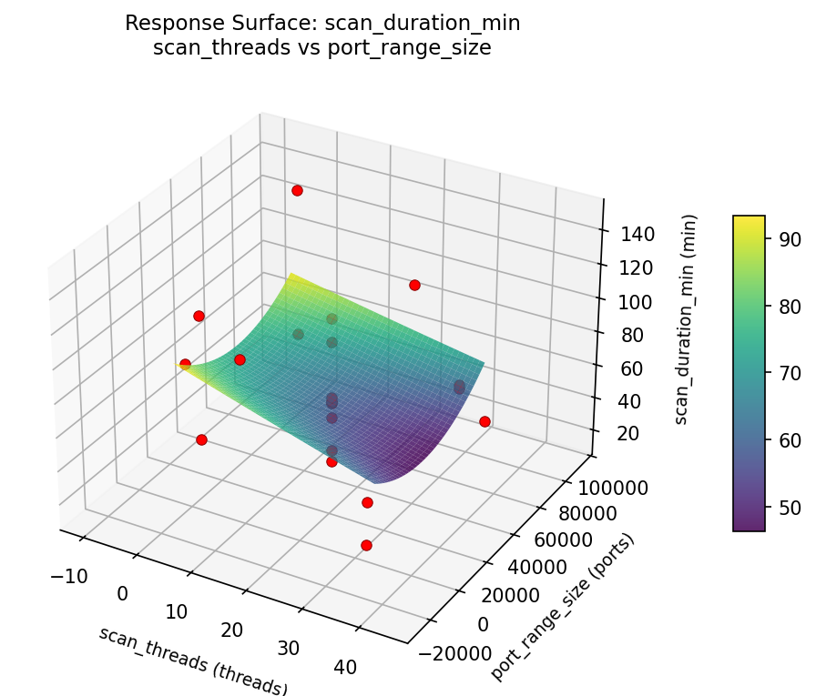
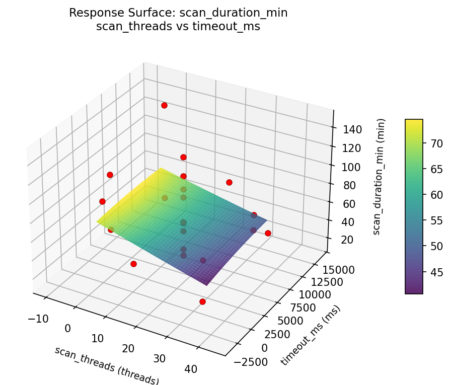
Response Surface Plots

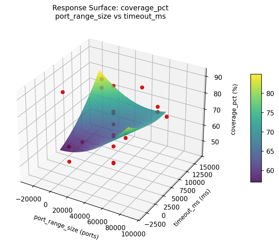
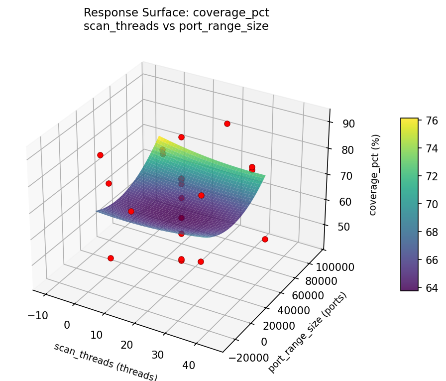
3D surfaces fitted with quadratic RSM. Red dots are observed data points.

coverage pct port range size vs timeout ms

coverage pct scan threads vs port range size

coverage pct scan threads vs timeout ms

scan duration min port range size vs timeout ms

scan duration min scan threads vs port range size

scan duration min scan threads vs timeout ms

Multi-Objective Optimization

When responses compete, Derringer–Suich desirability finds the best compromise. Each response is scaled to a 0–1 desirability, then combined via a weighted geometric mean.

Overall Desirability

D = 0.7874

Per-Response Desirability

Response	Weight	Desirability	Predicted	Dir
`scan_duration_min`	1.0	0.7780	40.50 0.7780 40.50 min	↓
`coverage_pct`	1.5	0.7938	82.90 0.7938 82.90 %	↑

Recommended Settings

Factor	Value
`scan_threads`	2 threads
`port_range_size`	100 ports
`timeout_ms`	10000 ms

Source: from observed run #2

Trade-off Summary

Sacrifice = how much worse than single-objective best.

Response	Predicted	Best Observed	Sacrifice
`coverage_pct`	82.90	91.30	+8.40

Top 3 Runs by Desirability

Run	D	Factor Settings
#10	0.7073	scan_threads=32, port_range_size=100, timeout_ms=10000
#18	0.6781	scan_threads=2, port_range_size=65535, timeout_ms=500

Model Quality

Response	R²	Type
`coverage_pct`	0.1506	linear

Full Multi-Objective Output

doe optimize --multi
============================================================
MULTI-OBJECTIVE OPTIMIZATION
Method: Derringer-Suich Desirability Function
============================================================

Overall desirability: D = 0.7874

Response                  Weight Desirability    Predicted  Direction
---------------------------------------------------------------------
scan_duration_min            1.0       0.7780       40.50 min   ↓
coverage_pct                 1.5       0.7938       82.90 %   ↑

Recommended settings:
  scan_threads = 2 threads
  port_range_size = 100 ports
  timeout_ms = 10000 ms
  (from observed run #2)

Trade-off summary:
  scan_duration_min: 40.50 (best observed: 14.60, sacrifice: +25.90)
  coverage_pct: 82.90 (best observed: 91.30, sacrifice: +8.40)

Model quality:
  scan_duration_min: R² = 0.1323 (linear)
  coverage_pct: R² = 0.1506 (linear)

Top 3 observed runs by overall desirability:
  1. Run #2 (D=0.7874): scan_threads=2, port_range_size=100, timeout_ms=10000
  2. Run #10 (D=0.7073): scan_threads=32, port_range_size=100, timeout_ms=10000
  3. Run #18 (D=0.6781): scan_threads=2, port_range_size=65535, timeout_ms=500

Full Analysis Output

doe analyze
=== Main Effects: scan_duration_min ===
Factor                   Effect    Std Error   % Contribution
--------------------------------------------------------------
port_range_size         98.1000       7.2297            53.9%
timeout_ms              68.0000       7.2297            37.4%
scan_threads            15.9500       7.2297             8.8%

=== ANOVA Table: scan_duration_min ===
Source                      DF           SS           MS          F    p-value
-----------------------------------------------------------------------------
scan_threads                 4     370.9970      92.7492      0.068     0.9901
port_range_size              4    7634.2395    1908.5599      1.400     0.3092
timeout_ms                   4    5171.2970    1292.8242      0.948     0.4797
Lack of Fit                  2    1426.4715     713.2357      0.523     0.6142
Pure Error                   7    9545.3587    1363.6227
Error                        9   10971.8302    1363.6227
Total                       21   24148.3636    1149.9221

=== Summary Statistics: scan_duration_min ===

scan_threads:
  Level               N       Mean        Std        Min        Max
  ------------------------------------------------------------
  -10.3861            1    58.5000     0.0000    58.5000    58.5000
  17                 12    66.8333    40.9081    14.6000   148.0000
  2                   4    70.7500    29.0065    40.5000   109.0000
  32                  4    74.4500    30.7951    56.3000   120.5000
  44.3861             1    59.7000     0.0000    59.7000    59.7000

port_range_size:
  Level               N       Mean        Std        Min        Max
  ------------------------------------------------------------
  -26916.2            1    49.9000     0.0000    49.9000    49.9000
  100                 4    71.6750    24.9996    56.3000   109.0000
  32817.5            12    60.1917    31.8012    14.6000   128.9000
  65535               4    73.5250    34.2283    40.5000   120.5000
  92551.2             1   148.0000     0.0000   148.0000   148.0000

timeout_ms:
  Level               N       Mean        Std        Min        Max
  ------------------------------------------------------------
  -3422.27            1    23.5000     0.0000    23.5000    23.5000
  10000               4    53.7000     8.8931    40.5000    59.2000
  13922.3             1    57.1000     0.0000    57.1000    57.1000
  500                 4    91.5000    27.6983    62.2000   120.5000
  5250               12    69.9667    38.6573    14.6000   148.0000

=== Main Effects: coverage_pct ===
Factor                   Effect    Std Error   % Contribution
--------------------------------------------------------------
port_range_size         27.9000       2.7406            52.5%
timeout_ms              17.7750       2.7406            33.4%
scan_threads             7.5000       2.7406            14.1%

=== ANOVA Table: coverage_pct ===
Source                      DF           SS           MS          F    p-value
-----------------------------------------------------------------------------
scan_threads                 4      47.7832      11.9458      0.054     0.9936
port_range_size              4     729.8632     182.4658      0.820     0.5441
timeout_ms                   4     757.3365     189.3341      0.850     0.5279
Lack of Fit                  2     376.5216     188.2608      0.846     0.4689
Pure Error                   7    1558.4688     222.6384
Error                        9    1934.9903     222.6384
Total                       21    3469.9732     165.2368

=== Summary Statistics: coverage_pct ===

scan_threads:
  Level               N       Mean        Std        Min        Max
  ------------------------------------------------------------
  -10.3861            1    68.3000     0.0000    68.3000    68.3000
  17                 12    69.5750    14.7693    43.8000    91.3000
  2                   4    68.6000    12.8206    54.5000    82.9000
  32                  4    68.5750    13.2872    48.7000    76.0000
  44.3861             1    75.8000     0.0000    75.8000    75.8000

port_range_size:
  Level               N       Mean        Std        Min        Max
  ------------------------------------------------------------
  -26916.2            1    44.3000     0.0000    44.3000    44.3000
  100                 4    69.8750    10.2902    54.5000    76.0000
  32817.5            12    71.8750    12.5431    43.8000    91.3000
  65535               4    67.3000    15.1857    48.7000    82.9000
  92551.2             1    72.2000     0.0000    72.2000    72.2000

timeout_ms:
  Level               N       Mean        Std        Min        Max
  ------------------------------------------------------------
  -3422.27            1    60.7000     0.0000    60.7000    60.7000
  10000               4    77.4750     3.6326    75.2000    82.9000
  13922.3             1    75.4000     0.0000    75.4000    75.4000
  500                 4    59.7000    10.8207    48.7000    73.8000
  5250               12    70.2417    14.5283    43.8000    91.3000

Optimization Recommendations

doe optimize
=== Optimization: scan_duration_min ===
Direction: minimize

Best observed run: #16
  scan_threads = 17
  port_range_size = 32817.5
  timeout_ms = 5250
  Value: 14.6

RSM Model (linear, R² = 0.0639, Adj R² = -0.0921):
  Coefficients:
    intercept                      +68.2273
    scan_threads                   -9.6108
    port_range_size                +0.5462
    timeout_ms                     +3.5414

RSM Model (quadratic, R² = 0.2014, Adj R² = -0.3976):
  Coefficients:
    intercept                      +66.0641
    scan_threads                   -9.6108
    port_range_size                +0.5462
    timeout_ms                     +3.5415
    scan_threads*port_range_size   -8.0250
    scan_threads*timeout_ms        -1.4250
    port_range_size*timeout_ms     +16.8500
    scan_threads^2                 +1.0516
    port_range_size^2              +4.3066
    timeout_ms^2                   -2.1134

  Curvature analysis:
    port_range_size                coef=+4.3066  convex (has a minimum)
    timeout_ms                     coef=-2.1134  concave (has a maximum)
    scan_threads                   coef=+1.0516  convex (has a minimum)

  Notable interactions:
    port_range_size*timeout_ms     coef=+16.8500  (synergistic)
    scan_threads*port_range_size   coef=-8.0250  (antagonistic)
    scan_threads*timeout_ms        coef=-1.4250  (antagonistic)

  Predicted optimum (from linear model, at observed points):
    scan_threads = -10.3861
    port_range_size = 32817.5
    timeout_ms = 5250
    Predicted value: 85.7740

  Surface optimum (via L-BFGS-B, linear model):
    scan_threads = 32
    port_range_size = 100
    timeout_ms = 500
    Predicted value: 54.5289

  Model quality: Weak fit — consider adding center points or using a different design.

Factor importance:
  1. timeout_ms  (effect: 38.7, contribution: 36.7%)
  2. scan_threads  (effect: 36.7, contribution: 34.9%)
  3. port_range_size  (effect: 29.9, contribution: 28.4%)

=== Optimization: coverage_pct ===
Direction: maximize

Best observed run: #18
  scan_threads = 17
  port_range_size = 32817.5
  timeout_ms = 5250
  Value: 91.3

RSM Model (linear, R² = 0.0886, Adj R² = -0.0633):
  Coefficients:
    intercept                      +69.4409
    scan_threads                   +4.0545
    port_range_size                +2.0951
    timeout_ms                     -0.3517

RSM Model (quadratic, R² = 0.1732, Adj R² = -0.4470):
  Coefficients:
    intercept                      +66.1659
    scan_threads                   +4.0545
    port_range_size                +2.0951
    timeout_ms                     -0.3517
    scan_threads*port_range_size   -3.6125
    scan_threads*timeout_ms        +1.0625
    port_range_size*timeout_ms     +1.5875
    scan_threads^2                 +0.7875
    port_range_size^2              +2.0475
    timeout_ms^2                   +2.0775

  Curvature analysis:
    timeout_ms                     coef=+2.0775  convex (has a minimum)
    port_range_size                coef=+2.0475  convex (has a minimum)
    scan_threads                   coef=+0.7875  convex (has a minimum)

  Notable interactions:
    scan_threads*port_range_size   coef=-3.6125  (antagonistic)
    port_range_size*timeout_ms     coef=+1.5875  (synergistic)
    scan_threads*timeout_ms        coef=+1.0625  (synergistic)

  Predicted optimum (from linear model, at observed points):
    scan_threads = 44.3861
    port_range_size = 32817.5
    timeout_ms = 5250
    Predicted value: 76.8434

  Surface optimum (via L-BFGS-B, linear model):
    scan_threads = 32
    port_range_size = 65535
    timeout_ms = 500
    Predicted value: 75.9422

  Model quality: Weak fit — consider adding center points or using a different design.

Factor importance:
  1. port_range_size  (effect: 21.0, contribution: 37.1%)
  2. timeout_ms  (effect: 17.9, contribution: 31.7%)
  3. scan_threads  (effect: 17.6, contribution: 31.2%)