Summary
This experiment investigates ble mesh topology. Box-Behnken design to tune relay count, TTL hops, and publish interval for message delivery and latency.
The design varies 3 factors: relay count (nodes), ranging from 2 to 10, ttl hops (hops), ranging from 2 to 8, and publish interval ms (ms), ranging from 100 to 2000. The goal is to optimize 2 responses: message delivery pct (%) (maximize) and network latency ms (ms) (minimize). Fixed conditions held constant across all runs include ble version = 5.0, mesh profile = sig_mesh.
A Box-Behnken design was chosen because it efficiently fits quadratic models with 3 continuous factors while avoiding extreme corner combinations — requiring only 15 runs instead of the 8 needed for a full factorial at two levels.
Quadratic response surface models were fitted to capture potential curvature and factor interactions. The RSM contour plots below visualize how pairs of factors jointly affect each response.
Key Findings
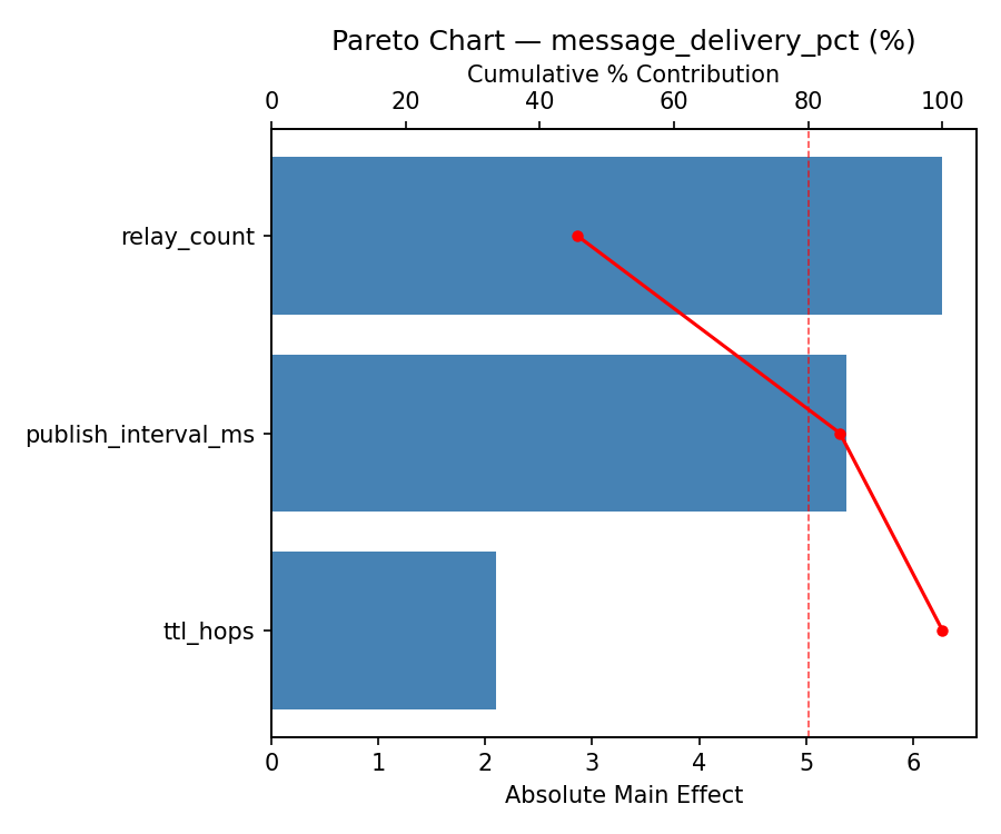
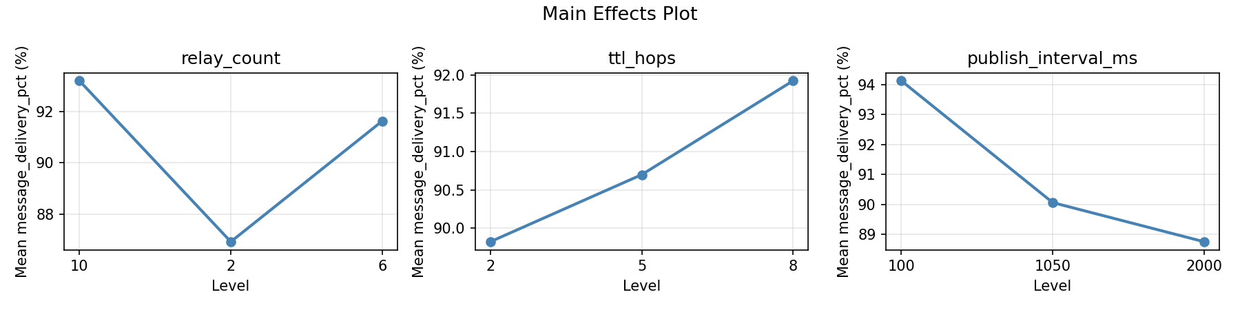
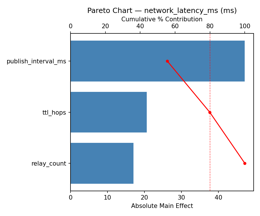
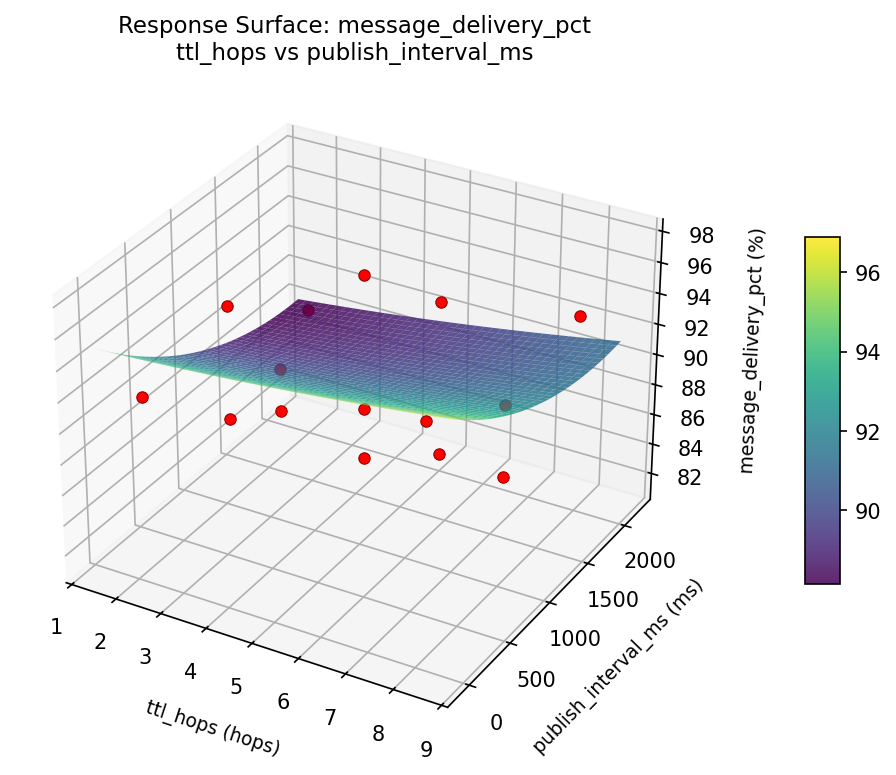
For message delivery pct, the most influential factors were publish interval ms (43.3%), ttl hops (39.4%), relay count (17.2%). The best observed value was 97.6 (at relay count = 2, ttl hops = 2, publish interval ms = 1050).
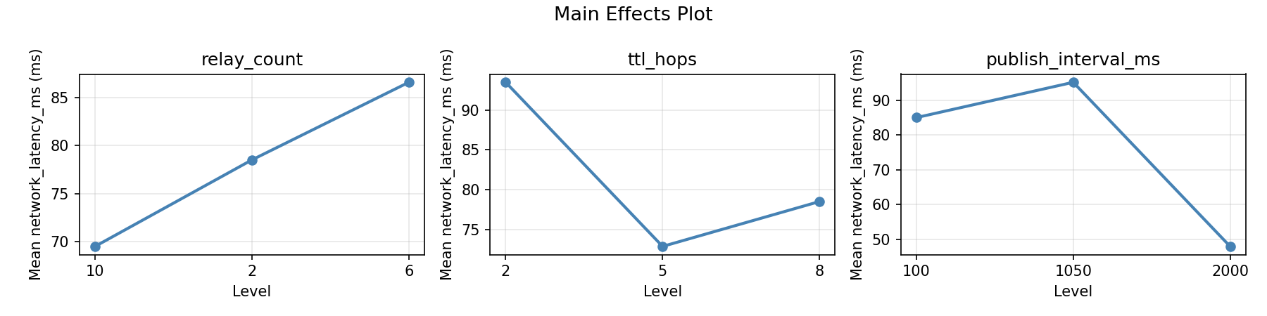
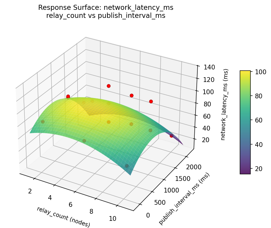
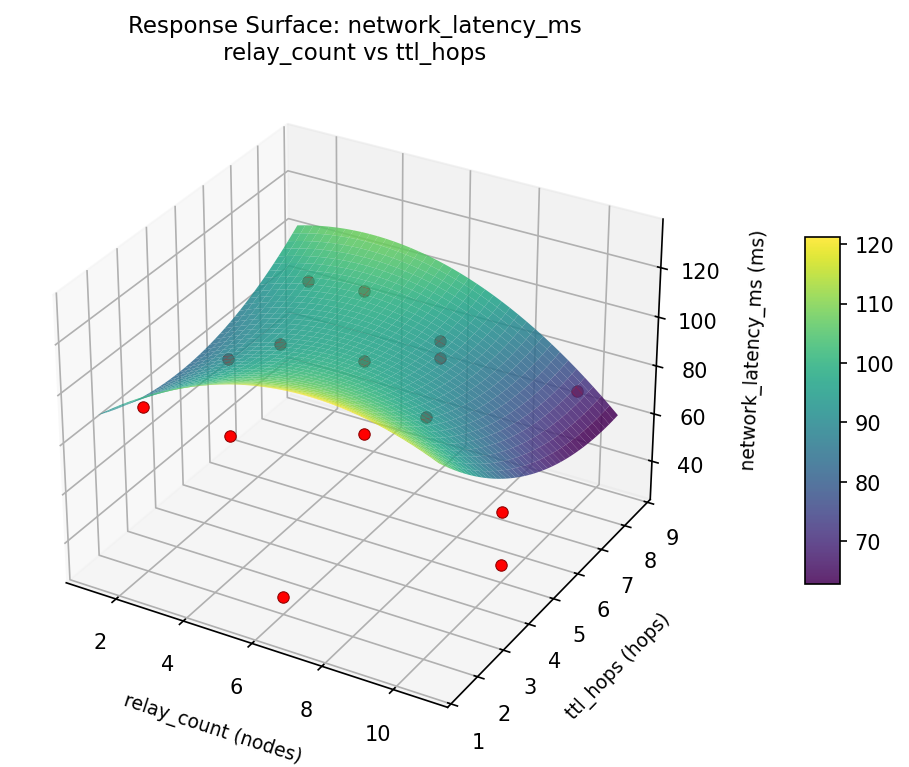
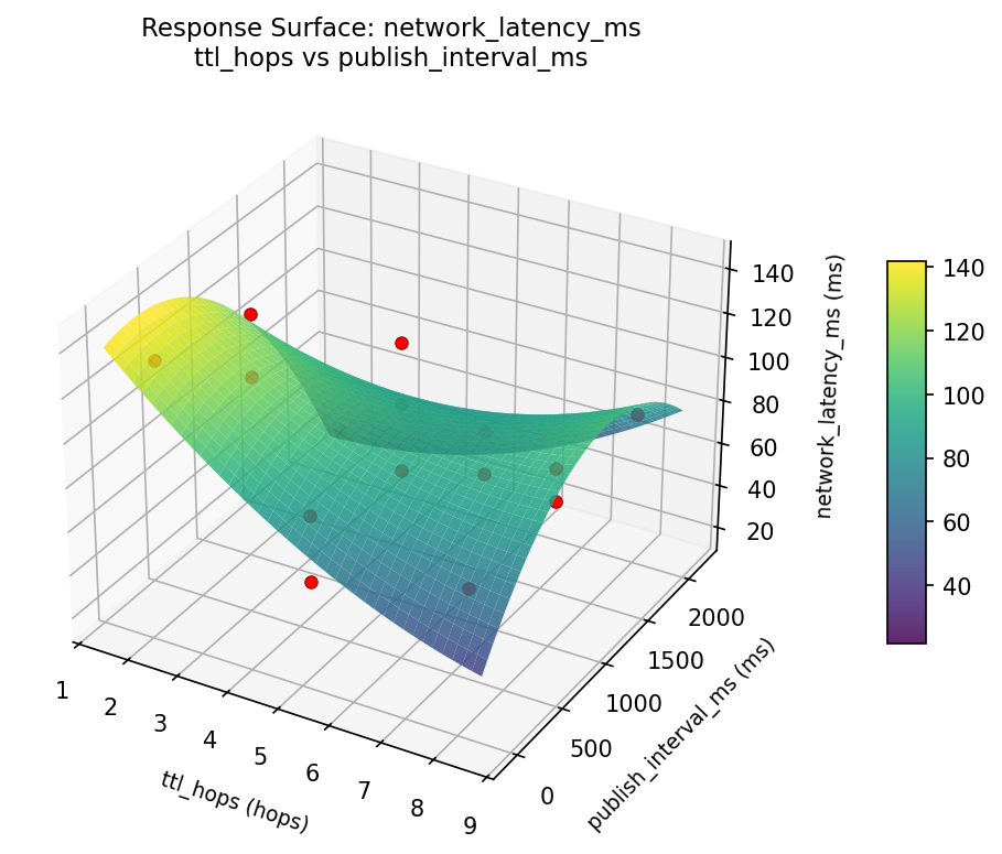
For network latency ms, the most influential factors were ttl hops (55.0%), relay count (27.7%), publish interval ms (17.3%). The best observed value was 31.0 (at relay count = 2, ttl hops = 8, publish interval ms = 1050).
Recommended Next Steps
- Run confirmation experiments at the predicted optimal settings to validate the model.
- Consider whether any fixed factors should be varied in a future study.
Experimental Setup
Factors
| Factor | Low | High | Unit |
|---|
relay_count | 2 | 10 | nodes |
ttl_hops | 2 | 8 | hops |
publish_interval_ms | 100 | 2000 | ms |
Fixed: ble_version = 5.0, mesh_profile = sig_mesh
Responses
| Response | Direction | Unit |
|---|
message_delivery_pct | ↑ maximize | % |
network_latency_ms | ↓ minimize | ms |
Configuration
{
"metadata": {
"name": "BLE Mesh Topology",
"description": "Box-Behnken design to tune relay count, TTL hops, and publish interval for message delivery and latency"
},
"factors": [
{
"name": "relay_count",
"levels": [
"2",
"10"
],
"type": "continuous",
"unit": "nodes"
},
{
"name": "ttl_hops",
"levels": [
"2",
"8"
],
"type": "continuous",
"unit": "hops"
},
{
"name": "publish_interval_ms",
"levels": [
"100",
"2000"
],
"type": "continuous",
"unit": "ms"
}
],
"fixed_factors": {
"ble_version": "5.0",
"mesh_profile": "sig_mesh"
},
"responses": [
{
"name": "message_delivery_pct",
"optimize": "maximize",
"unit": "%"
},
{
"name": "network_latency_ms",
"optimize": "minimize",
"unit": "ms"
}
],
"settings": {
"operation": "box_behnken",
"test_script": "use_cases/68_ble_mesh_topology/sim.sh"
}
}
Experimental Matrix
The Box-Behnken Design produces 15 runs. Each row is one experiment with specific factor settings.
| Run | relay_count | ttl_hops | publish_interval_ms |
|---|
| 1 | 6 | 2 | 100 |
| 2 | 6 | 5 | 1050 |
| 3 | 10 | 5 | 2000 |
| 4 | 10 | 5 | 100 |
| 5 | 6 | 5 | 1050 |
| 6 | 6 | 5 | 1050 |
| 7 | 2 | 5 | 2000 |
| 8 | 10 | 2 | 1050 |
| 9 | 6 | 2 | 2000 |
| 10 | 10 | 8 | 1050 |
| 11 | 2 | 5 | 100 |
| 12 | 6 | 8 | 2000 |
| 13 | 2 | 2 | 1050 |
| 14 | 2 | 8 | 1050 |
| 15 | 6 | 8 | 100 |
Step-by-Step Workflow
1
Preview the design
$ doe info --config use_cases/68_ble_mesh_topology/config.json
2
Generate the runner script
$ doe generate --config use_cases/68_ble_mesh_topology/config.json \
--output use_cases/68_ble_mesh_topology/results/run.sh --seed 42
3
Execute the experiments
$ bash use_cases/68_ble_mesh_topology/results/run.sh
4
Analyze results
$ doe analyze --config use_cases/68_ble_mesh_topology/config.json
5
Get optimization recommendations
$ doe optimize --config use_cases/68_ble_mesh_topology/config.json
6
Multi-objective optimization
With 2 competing responses, use --multi to find the best compromise via Derringer–Suich desirability.
$ doe optimize --config use_cases/68_ble_mesh_topology/config.json --multi
7
Generate the HTML report
$ doe report --config use_cases/68_ble_mesh_topology/config.json \
--output use_cases/68_ble_mesh_topology/results/report.html
Features Exercised
| Feature | Value |
|---|
| Design type | box_behnken |
| Factor types | continuous (all 3) |
| Arg style | double-dash |
| Responses | 2 (message_delivery_pct ↑, network_latency_ms ↓) |
| Total runs | 15 |
Analysis Results
Generated from actual experiment runs using the DOE Helper Tool.
Response: message_delivery_pct
Top factors: publish_interval_ms (43.3%), ttl_hops (39.4%), relay_count (17.2%).
ANOVA
| Source | DF | SS | MS | F | p-value |
|---|
| Source | DF | SS | MS | F | p-value |
| relay_count | 2 | 3.3200 | 1.6600 | 0.025 | 0.9758 |
| ttl_hops | 2 | 24.7822 | 12.3911 | 0.183 | 0.8358 |
| publish_interval_ms | 2 | 25.5022 | 12.7511 | 0.189 | 0.8315 |
| Lack | of | Fit | 6 | 86.8649 | 14.4775 |
| Pure | Error | 2 | 135.0600 | | |
| Error | 8 | 221.9249 | 67.5300 | | |
| Total | 14 | 275.5293 | 19.6807 | | |
Pareto Chart
Main Effects Plot
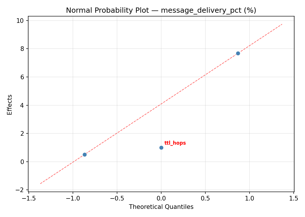
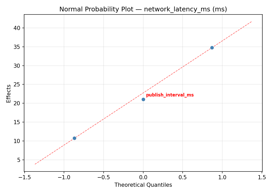
Normal Probability Plot of Effects
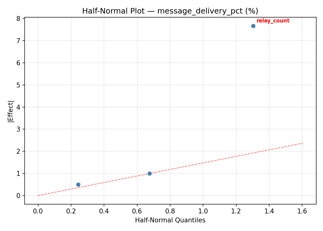
Half-Normal Plot of Effects
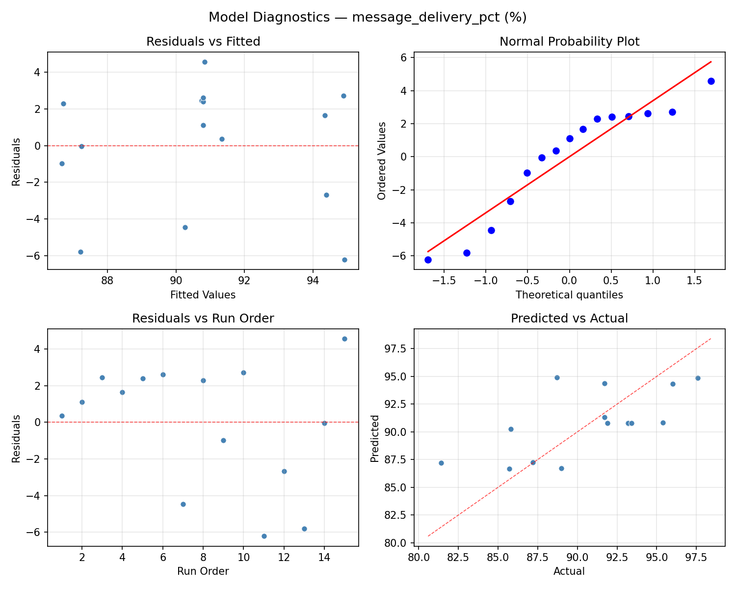
Model Diagnostics
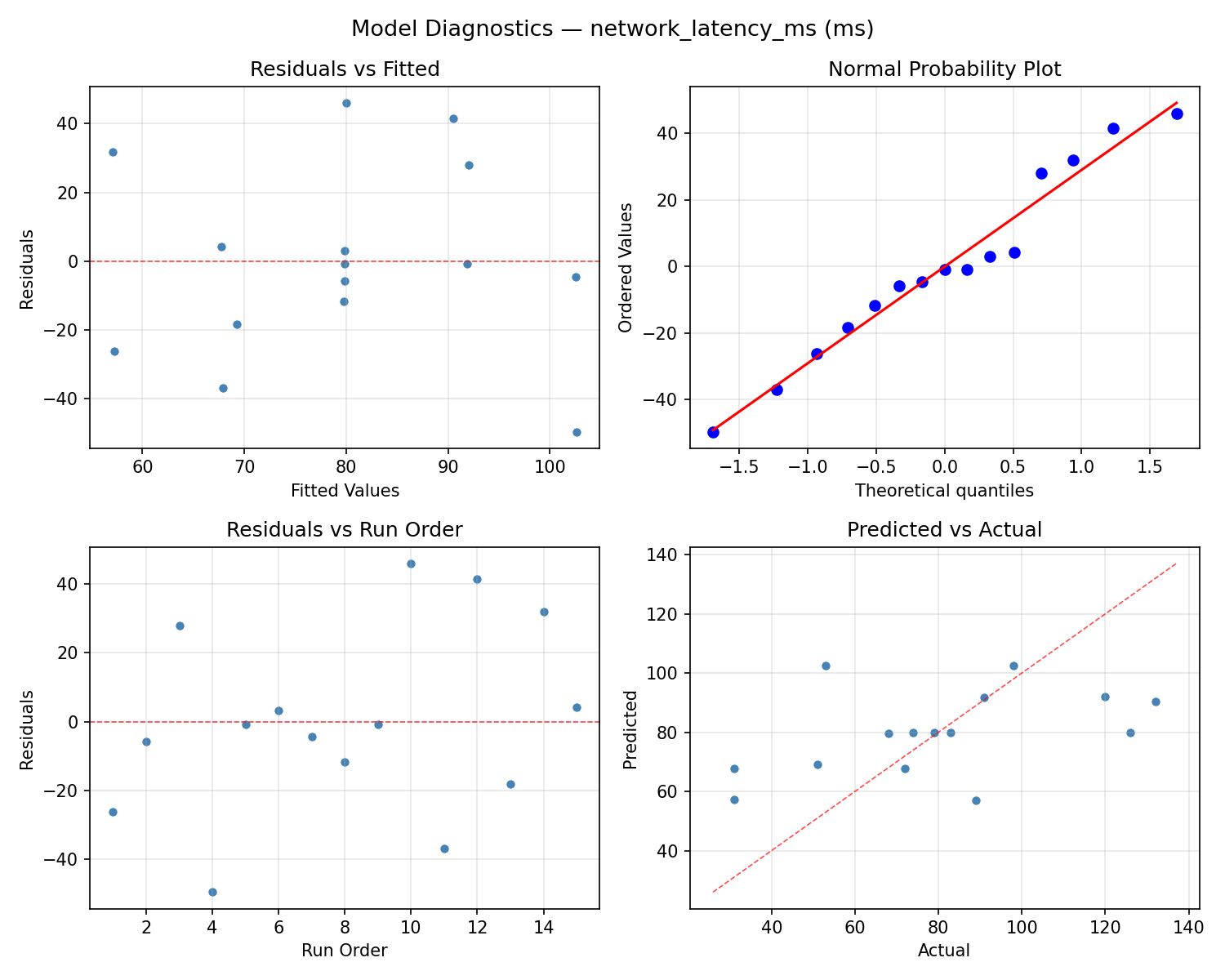
Response: network_latency_ms
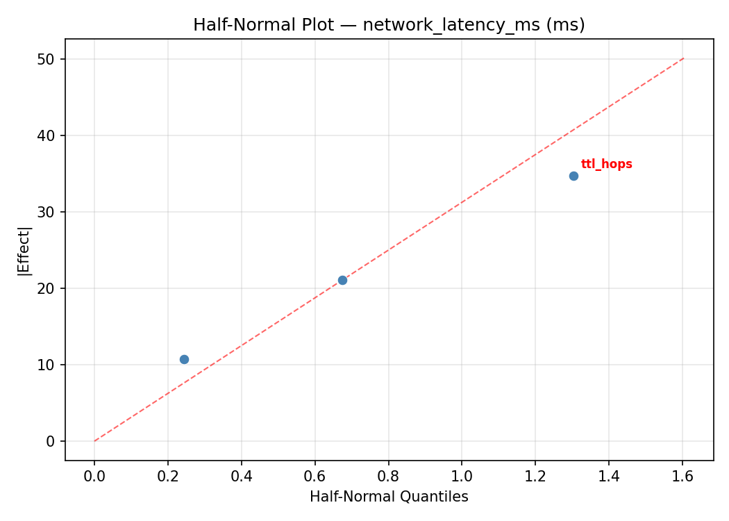
Top factors: ttl_hops (55.0%), relay_count (27.7%), publish_interval_ms (17.3%).
ANOVA
| Source | DF | SS | MS | F | p-value |
|---|
| Source | DF | SS | MS | F | p-value |
| relay_count | 2 | 1337.5548 | 668.7774 | 0.453 | 0.6511 |
| ttl_hops | 2 | 4185.2690 | 2092.6345 | 1.417 | 0.2972 |
| publish_interval_ms | 2 | 608.0190 | 304.0095 | 0.206 | 0.8181 |
| Lack | of | Fit | 6 | 4488.2238 | 748.0373 |
| Pure | Error | 2 | 2952.6667 | | |
| Error | 8 | 7440.8905 | 1476.3333 | | |
| Total | 14 | 13571.7333 | 969.4095 | | |
Pareto Chart
Main Effects Plot
Normal Probability Plot of Effects
Half-Normal Plot of Effects
Model Diagnostics
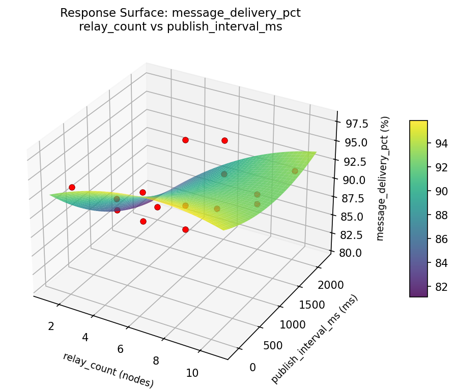
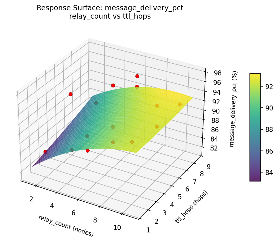
Response Surface Plots
3D surfaces fitted with quadratic RSM. Red dots are observed data points.
message delivery pct relay count vs publish interval ms
message delivery pct relay count vs ttl hops
message delivery pct ttl hops vs publish interval ms
network latency ms relay count vs publish interval ms
network latency ms relay count vs ttl hops
network latency ms ttl hops vs publish interval ms
Multi-Objective Optimization
When responses compete, Derringer–Suich desirability finds the best compromise.
Each response is scaled to a 0–1 desirability, then combined via a weighted geometric mean.
Overall Desirability
D = 0.8197
Per-Response Desirability
| Response | Weight | Desirability | Predicted | Dir |
|---|
message_delivery_pct |
1.5 |
|
96.00 0.8648 96.00 % |
↑ |
network_latency_ms |
1.0 |
|
53.00 0.7565 53.00 ms |
↓ |
Recommended Settings
| Factor | Value |
|---|
relay_count | 2 nodes |
ttl_hops | 5 hops |
publish_interval_ms | 100 ms |
Source: from observed run #4
Trade-off Summary
Sacrifice = how much worse than single-objective best.
| Response | Predicted | Best Observed | Sacrifice |
|---|
network_latency_ms | 53.00 | 31.00 | +22.00 |
Top 3 Runs by Desirability
| Run | D | Factor Settings |
|---|
| #1 | 0.7393 | relay_count=2, ttl_hops=2, publish_interval_ms=1050 |
| #15 | 0.7224 | relay_count=10, ttl_hops=2, publish_interval_ms=1050 |
Model Quality
| Response | R² | Type |
|---|
network_latency_ms | 0.7153 | quadratic |
Full Multi-Objective Output
============================================================
MULTI-OBJECTIVE OPTIMIZATION
Method: Derringer-Suich Desirability Function
============================================================
Overall desirability: D = 0.8197
Response Weight Desirability Predicted Direction
---------------------------------------------------------------------
message_delivery_pct 1.5 0.8648 96.00 % ↑
network_latency_ms 1.0 0.7565 53.00 ms ↓
Recommended settings:
relay_count = 2 nodes
ttl_hops = 5 hops
publish_interval_ms = 100 ms
(from observed run #4)
Trade-off summary:
message_delivery_pct: 96.00 (best observed: 97.60, sacrifice: +1.60)
network_latency_ms: 53.00 (best observed: 31.00, sacrifice: +22.00)
Model quality:
message_delivery_pct: R² = 0.2199 (linear)
network_latency_ms: R² = 0.7153 (quadratic)
Top 3 observed runs by overall desirability:
1. Run #4 (D=0.8197): relay_count=2, ttl_hops=5, publish_interval_ms=100
2. Run #1 (D=0.7393): relay_count=2, ttl_hops=2, publish_interval_ms=1050
3. Run #15 (D=0.7224): relay_count=10, ttl_hops=2, publish_interval_ms=1050
Full Analysis Output
=== Main Effects: message_delivery_pct ===
Factor Effect Std Error % Contribution
--------------------------------------------------------------
publish_interval_ms 3.1429 1.1454 43.3%
ttl_hops 2.8571 1.1454 39.4%
relay_count 1.2500 1.1454 17.2%
=== ANOVA Table: message_delivery_pct ===
Source DF SS MS F p-value
-----------------------------------------------------------------------------
relay_count 2 3.3200 1.6600 0.025 0.9758
ttl_hops 2 24.7822 12.3911 0.183 0.8358
publish_interval_ms 2 25.5022 12.7511 0.189 0.8315
Lack of Fit 6 86.8649 14.4775 0.214 0.9400
Pure Error 2 135.0600 67.5300
Error 8 221.9249 67.5300
Total 14 275.5293 19.6807
=== Summary Statistics: message_delivery_pct ===
relay_count:
Level N Mean Std Min Max
------------------------------------------------------------
10 4 90.2750 2.6875 87.2000 93.2000
2 4 91.5250 4.1080 85.8000 95.4000
6 7 90.6714 5.7723 81.4000 97.6000
ttl_hops:
Level N Mean Std Min Max
------------------------------------------------------------
2 4 91.6500 4.3486 85.7000 96.0000
5 7 89.4429 5.3210 81.4000 97.6000
8 4 92.3000 2.8367 88.7000 95.4000
publish_interval_ms:
Level N Mean Std Min Max
------------------------------------------------------------
100 4 91.0500 4.5384 85.8000 96.0000
1050 7 91.8429 5.1111 81.4000 97.6000
2000 4 88.7000 3.2404 85.7000 93.2000
=== Main Effects: network_latency_ms ===
Factor Effect Std Error % Contribution
--------------------------------------------------------------
ttl_hops 44.7500 8.0391 55.0%
relay_count 22.5357 8.0391 27.7%
publish_interval_ms 14.0714 8.0391 17.3%
=== ANOVA Table: network_latency_ms ===
Source DF SS MS F p-value
-----------------------------------------------------------------------------
relay_count 2 1337.5548 668.7774 0.453 0.6511
ttl_hops 2 4185.2690 2092.6345 1.417 0.2972
publish_interval_ms 2 608.0190 304.0095 0.206 0.8181
Lack of Fit 6 4488.2238 748.0373 0.507 0.7805
Pure Error 2 2952.6667 1476.3333
Error 8 7440.8905 1476.3333
Total 14 13571.7333 969.4095
=== Summary Statistics: network_latency_ms ===
relay_count:
Level N Mean Std Min Max
------------------------------------------------------------
10 4 77.0000 37.3720 31.0000 120.0000
2 4 95.2500 26.8499 72.0000 132.0000
6 7 72.7143 31.3088 31.0000 126.0000
ttl_hops:
Level N Mean Std Min Max
------------------------------------------------------------
2 4 99.0000 35.1663 53.0000 132.0000
5 7 83.5714 23.9921 51.0000 126.0000
8 4 54.2500 27.2198 31.0000 83.0000
publish_interval_ms:
Level N Mean Std Min Max
------------------------------------------------------------
100 4 75.5000 19.3649 53.0000 98.0000
1050 7 86.5714 39.7067 31.0000 132.0000
2000 4 72.5000 28.1603 31.0000 91.0000
Optimization Recommendations
=== Optimization: message_delivery_pct ===
Direction: maximize
Best observed run: #10
relay_count = 2
ttl_hops = 2
publish_interval_ms = 1050
Value: 97.6
RSM Model (linear, R² = 0.2148, Adj R² = 0.0006):
Coefficients:
intercept +90.7933
relay_count -1.6750
ttl_hops -0.7000
publish_interval_ms +2.0250
RSM Model (quadratic, R² = 0.6238, Adj R² = -0.0535):
Coefficients:
intercept +94.0000
relay_count -1.6750
ttl_hops -0.7000
publish_interval_ms +2.0250
relay_count*ttl_hops +1.9250
relay_count*publish_interval_ms +2.1250
ttl_hops*publish_interval_ms -2.6250
relay_count^2 -1.8375
ttl_hops^2 -0.7875
publish_interval_ms^2 -3.3875
Curvature analysis:
publish_interval_ms coef=-3.3875 concave (has a maximum)
relay_count coef=-1.8375 concave (has a maximum)
ttl_hops coef=-0.7875 concave (has a maximum)
Notable interactions:
ttl_hops*publish_interval_ms coef=-2.6250 (antagonistic)
relay_count*publish_interval_ms coef=+2.1250 (synergistic)
relay_count*ttl_hops coef=+1.9250 (synergistic)
Predicted optimum (from linear model, at observed points):
relay_count = 2
ttl_hops = 5
publish_interval_ms = 2000
Predicted value: 94.4933
Surface optimum (via L-BFGS-B, linear model):
relay_count = 2
ttl_hops = 2
publish_interval_ms = 2000
Predicted value: 95.1933
Model quality: Weak fit — consider adding center points or using a different design.
Factor importance:
1. publish_interval_ms (effect: 5.2, contribution: 52.4%)
2. relay_count (effect: 3.3, contribution: 33.6%)
3. ttl_hops (effect: 1.4, contribution: 14.0%)
=== Optimization: network_latency_ms ===
Direction: minimize
Best observed run: #1
relay_count = 2
ttl_hops = 8
publish_interval_ms = 1050
Value: 31.0
RSM Model (linear, R² = 0.1082, Adj R² = -0.1350):
Coefficients:
intercept +79.8667
relay_count -8.5000
ttl_hops -8.5000
publish_interval_ms +6.2500
RSM Model (quadratic, R² = 0.6237, Adj R² = -0.0535):
Coefficients:
intercept +78.0000
relay_count -8.5000
ttl_hops -8.5000
publish_interval_ms +6.2500
relay_count*ttl_hops +18.5000
relay_count*publish_interval_ms +6.5000
ttl_hops*publish_interval_ms -32.5000
relay_count^2 -12.0000
ttl_hops^2 +12.5000
publish_interval_ms^2 +3.0000
Curvature analysis:
ttl_hops coef=+12.5000 convex (has a minimum)
relay_count coef=-12.0000 concave (has a maximum)
publish_interval_ms coef=+3.0000 convex (has a minimum)
Notable interactions:
ttl_hops*publish_interval_ms coef=-32.5000 (antagonistic)
relay_count*ttl_hops coef=+18.5000 (synergistic)
relay_count*publish_interval_ms coef=+6.5000 (synergistic)
Predicted optimum (from quadratic model, at observed points):
relay_count = 6
ttl_hops = 2
publish_interval_ms = 2000
Predicted value: 140.7500
Surface optimum (via L-BFGS-B, quadratic model):
relay_count = 10
ttl_hops = 2
publish_interval_ms = 100
Predicted value: 17.7500
Model quality: Moderate fit — use predictions directionally, not precisely.
Factor importance:
1. ttl_hops (effect: 21.6, contribution: 38.8%)
2. relay_count (effect: 21.6, contribution: 38.8%)
3. publish_interval_ms (effect: 12.5, contribution: 22.4%)