Summary
This experiment investigates lorawan parameters. Central Composite design to optimize spreading factor, TX power, and coding rate for range and battery life.
The design varies 3 factors: spreading factor (SF), ranging from 7 to 12, tx power dbm (dBm), ranging from 2 to 20, and coding rate (CR), ranging from 5 to 8. The goal is to optimize 2 responses: range km (km) (maximize) and battery life days (days) (maximize). Fixed conditions held constant across all runs include frequency = 915MHz, bandwidth = 125kHz.
A Central Composite Design (CCD) was selected to fit a full quadratic response surface model, including curvature and interaction effects. With 3 factors this produces 22 runs including center points and axial (star) points that extend beyond the factorial range.
Quadratic response surface models were fitted to capture potential curvature and factor interactions. The RSM contour plots below visualize how pairs of factors jointly affect each response.
Key Findings
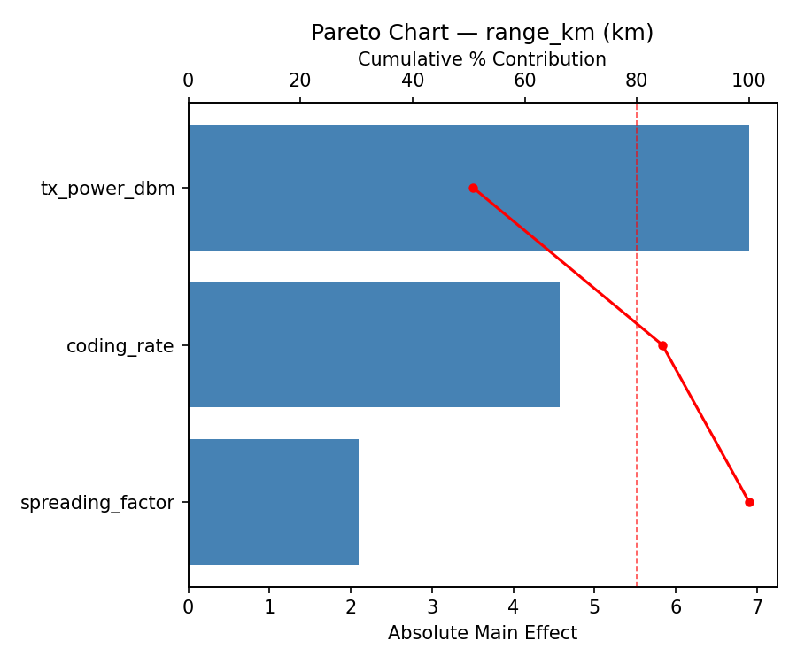
For range km, the most influential factors were tx power dbm (51.7%), coding rate (43.4%), spreading factor (4.8%). The best observed value was 10.9 (at spreading factor = 9.5, tx power dbm = 11, coding rate = 3.76139).
For battery life days, the most influential factors were tx power dbm (51.2%), coding rate (39.4%), spreading factor (9.4%). The best observed value was 554.0 (at spreading factor = 14.0644, tx power dbm = 11, coding rate = 6.5).
Recommended Next Steps
- Run confirmation experiments at the predicted optimal settings to validate the model.
- Consider whether any fixed factors should be varied in a future study.
Experimental Setup
Factors
| Factor | Low | High | Unit |
|---|
spreading_factor | 7 | 12 | SF |
tx_power_dbm | 2 | 20 | dBm |
coding_rate | 5 | 8 | CR |
Fixed: frequency = 915MHz, bandwidth = 125kHz
Responses
| Response | Direction | Unit |
|---|
range_km | ↑ maximize | km |
battery_life_days | ↑ maximize | days |
Configuration
{
"metadata": {
"name": "LoRaWAN Parameters",
"description": "Central Composite design to optimize spreading factor, TX power, and coding rate for range and battery life"
},
"factors": [
{
"name": "spreading_factor",
"levels": [
"7",
"12"
],
"type": "continuous",
"unit": "SF"
},
{
"name": "tx_power_dbm",
"levels": [
"2",
"20"
],
"type": "continuous",
"unit": "dBm"
},
{
"name": "coding_rate",
"levels": [
"5",
"8"
],
"type": "continuous",
"unit": "CR"
}
],
"fixed_factors": {
"frequency": "915MHz",
"bandwidth": "125kHz"
},
"responses": [
{
"name": "range_km",
"optimize": "maximize",
"unit": "km"
},
{
"name": "battery_life_days",
"optimize": "maximize",
"unit": "days"
}
],
"settings": {
"operation": "central_composite",
"test_script": "use_cases/70_lorawan_parameters/sim.sh"
}
}
Experimental Matrix
The Central Composite Design produces 22 runs. Each row is one experiment with specific factor settings.
| Run | spreading_factor | tx_power_dbm | coding_rate |
|---|
| 1 | 9.5 | 11 | 6.5 |
| 2 | 12 | 2 | 8 |
| 3 | 7 | 20 | 5 |
| 4 | 9.5 | 27.4317 | 6.5 |
| 5 | 9.5 | 11 | 6.5 |
| 6 | 4.93565 | 11 | 6.5 |
| 7 | 9.5 | 11 | 3.76139 |
| 8 | 9.5 | 11 | 6.5 |
| 9 | 12 | 20 | 5 |
| 10 | 14.0644 | 11 | 6.5 |
| 11 | 9.5 | 11 | 6.5 |
| 12 | 9.5 | -5.43168 | 6.5 |
| 13 | 9.5 | 11 | 6.5 |
| 14 | 7 | 2 | 8 |
| 15 | 9.5 | 11 | 6.5 |
| 16 | 12 | 2 | 5 |
| 17 | 9.5 | 11 | 9.23861 |
| 18 | 12 | 20 | 8 |
| 19 | 9.5 | 11 | 6.5 |
| 20 | 7 | 2 | 5 |
| 21 | 7 | 20 | 8 |
| 22 | 9.5 | 11 | 6.5 |
Step-by-Step Workflow
1
Preview the design
$ doe info --config use_cases/70_lorawan_parameters/config.json
2
Generate the runner script
$ doe generate --config use_cases/70_lorawan_parameters/config.json \
--output use_cases/70_lorawan_parameters/results/run.sh --seed 42
3
Execute the experiments
$ bash use_cases/70_lorawan_parameters/results/run.sh
4
Analyze results
$ doe analyze --config use_cases/70_lorawan_parameters/config.json
5
Get optimization recommendations
$ doe optimize --config use_cases/70_lorawan_parameters/config.json
6
Multi-objective optimization
With 2 competing responses, use --multi to find the best compromise via Derringer–Suich desirability.
$ doe optimize --config use_cases/70_lorawan_parameters/config.json --multi
7
Generate the HTML report
$ doe report --config use_cases/70_lorawan_parameters/config.json \
--output use_cases/70_lorawan_parameters/results/report.html
Features Exercised
| Feature | Value |
|---|
| Design type | central_composite |
| Factor types | continuous (all 3) |
| Arg style | double-dash |
| Responses | 2 (range_km ↑, battery_life_days ↑) |
| Total runs | 22 |
Analysis Results
Generated from actual experiment runs using the DOE Helper Tool.
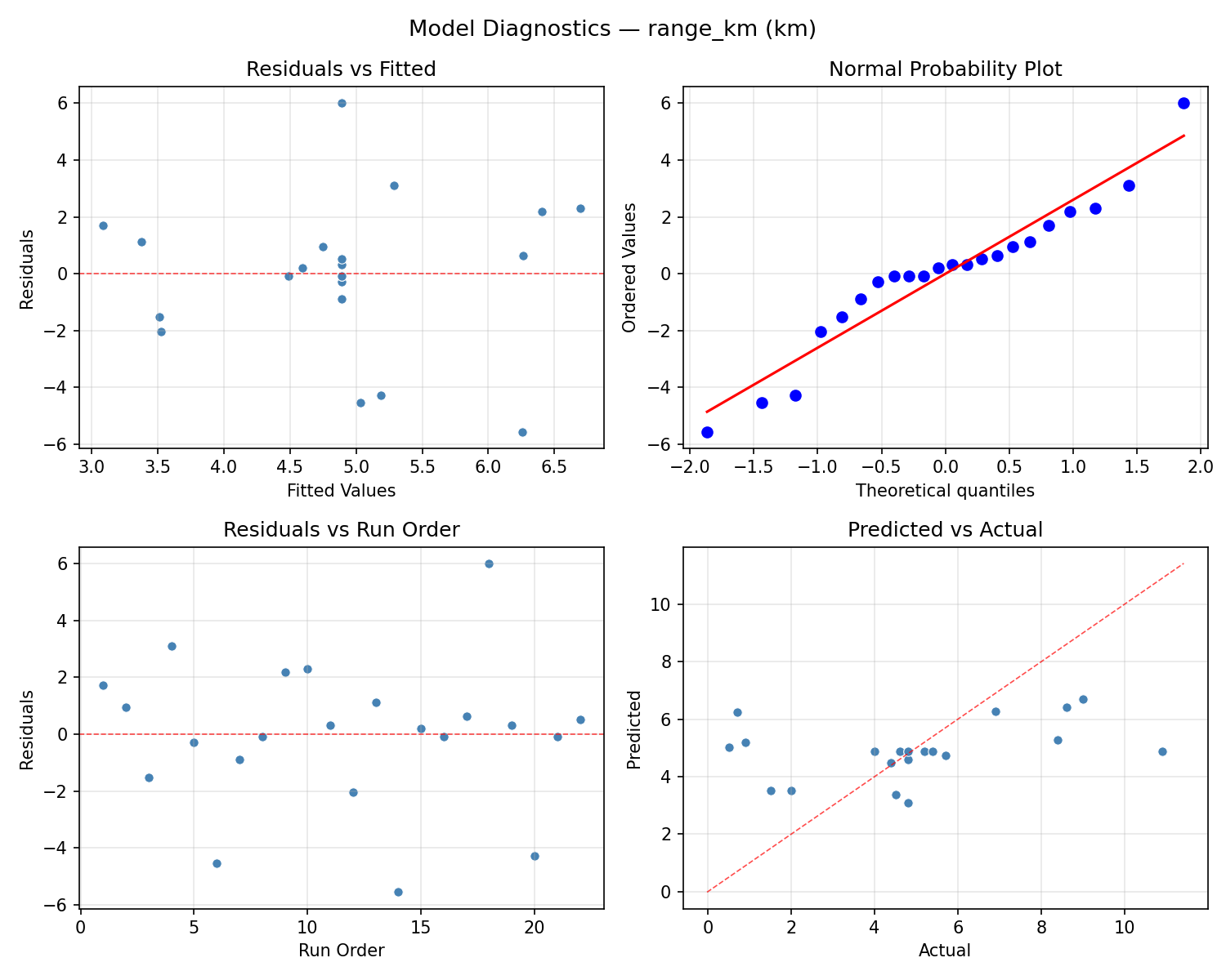
Response: range_km
Top factors: tx_power_dbm (51.7%), coding_rate (43.4%), spreading_factor (4.8%).
ANOVA
| Source | DF | SS | MS | F | p-value |
|---|
| Source | DF | SS | MS | F | p-value |
| spreading_factor | 4 | 1.2715 | 0.3179 | 0.035 | 0.9972 |
| tx_power_dbm | 4 | 40.4840 | 10.1210 | 1.113 | 0.4080 |
| coding_rate | 4 | 33.4807 | 8.3702 | 0.920 | 0.4929 |
| Lack | of | Fit | 2 | 19.2432 | 9.6216 |
| Pure | Error | 7 | 63.6588 | | |
| Error | 9 | 82.9020 | 9.0941 | | |
| Total | 21 | 158.1382 | 7.5304 | | |
Pareto Chart
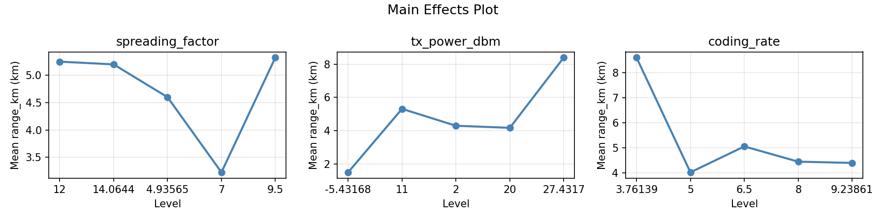
Main Effects Plot
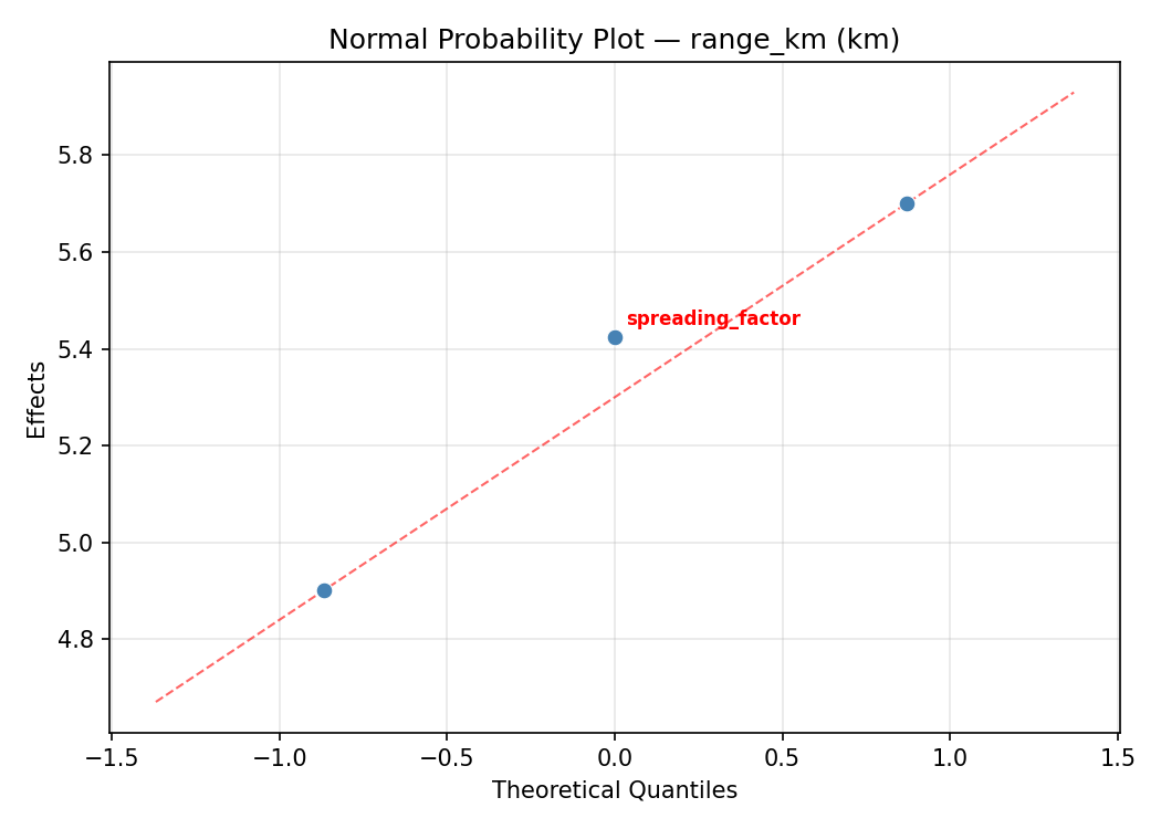
Normal Probability Plot of Effects
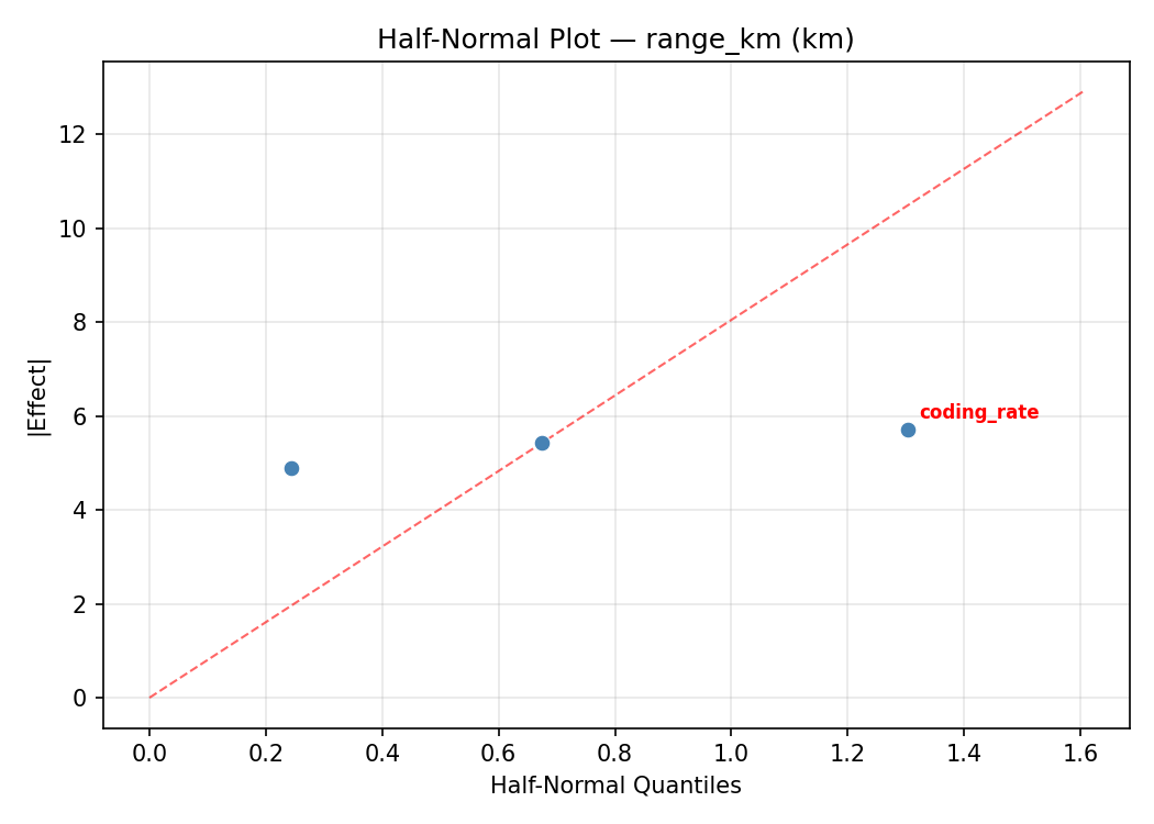
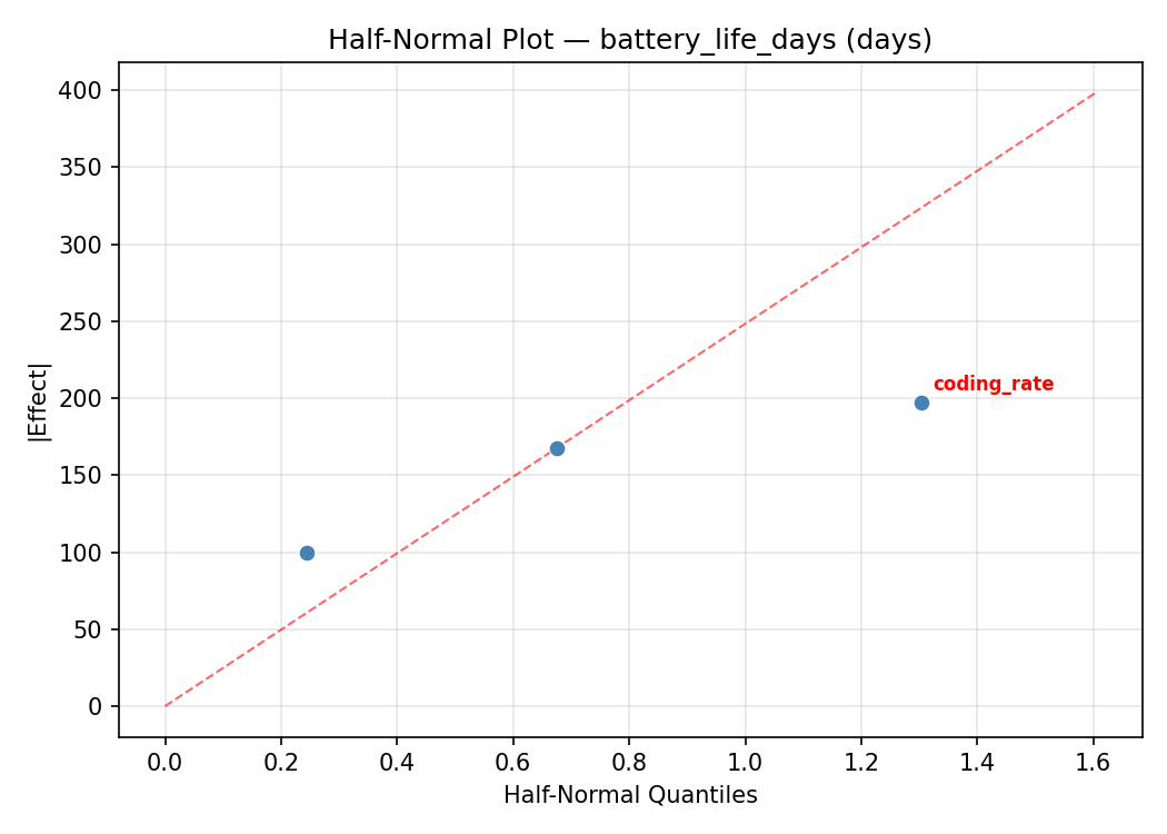
Half-Normal Plot of Effects
Model Diagnostics
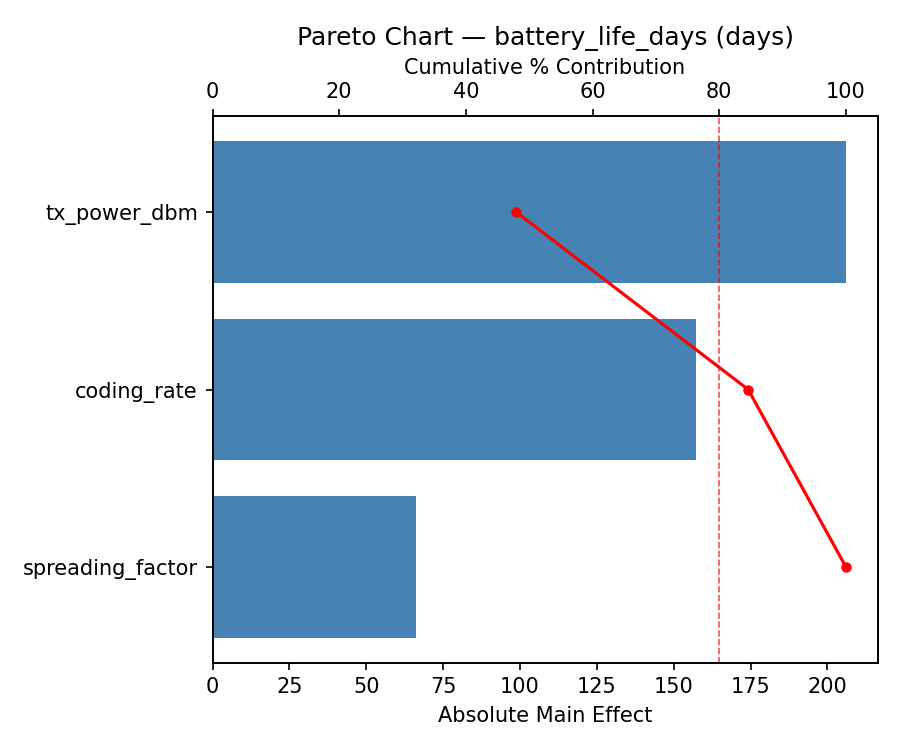
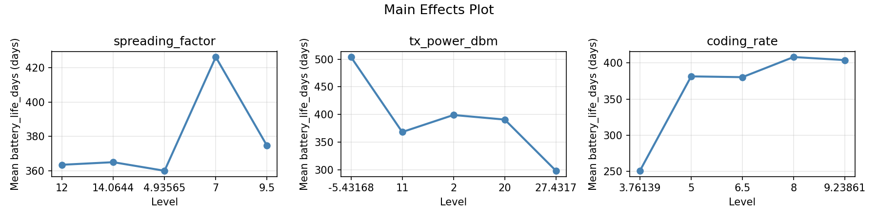
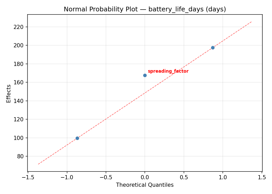
Response: battery_life_days
Top factors: tx_power_dbm (51.2%), coding_rate (39.4%), spreading_factor (9.4%).
ANOVA
| Source | DF | SS | MS | F | p-value |
|---|
| Source | DF | SS | MS | F | p-value |
| spreading_factor | 4 | 2503.5909 | 625.8977 | 0.084 | 0.9852 |
| tx_power_dbm | 4 | 46473.5909 | 11618.3977 | 1.564 | 0.2646 |
| coding_rate | 4 | 28375.6742 | 7093.9186 | 0.955 | 0.4764 |
| Lack | of | Fit | 2 | 22630.8598 | 11315.4299 |
| Pure | Error | 7 | 51992.8750 | | |
| Error | 9 | 74623.7348 | 7427.5536 | | |
| Total | 21 | 151976.5909 | 7236.9805 | | |
Pareto Chart
Main Effects Plot
Normal Probability Plot of Effects
Half-Normal Plot of Effects
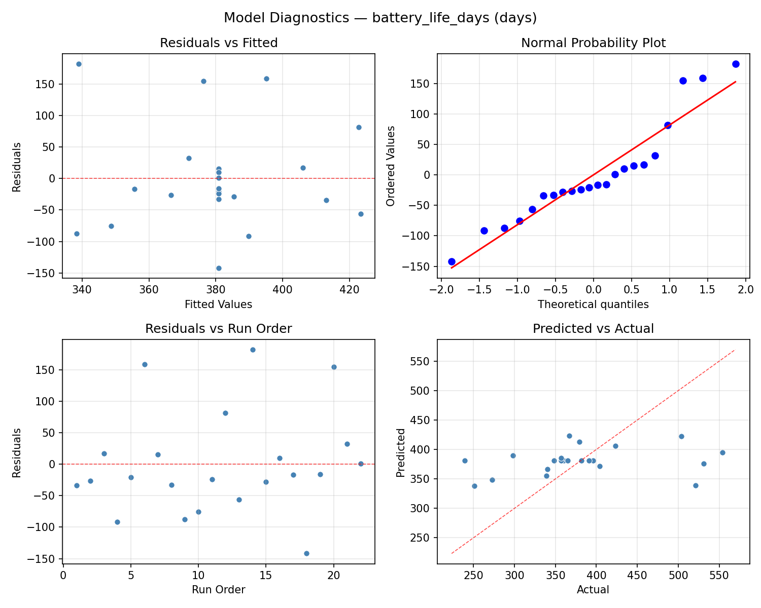
Model Diagnostics
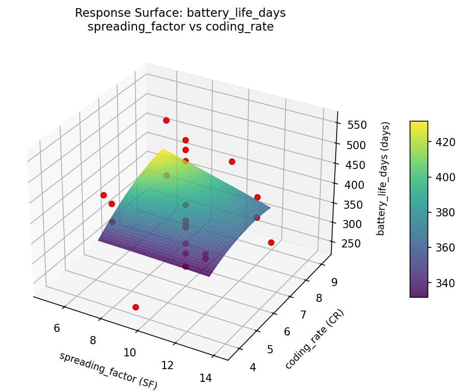
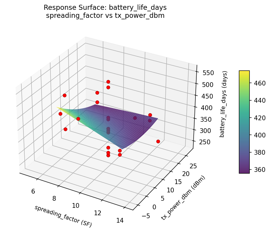
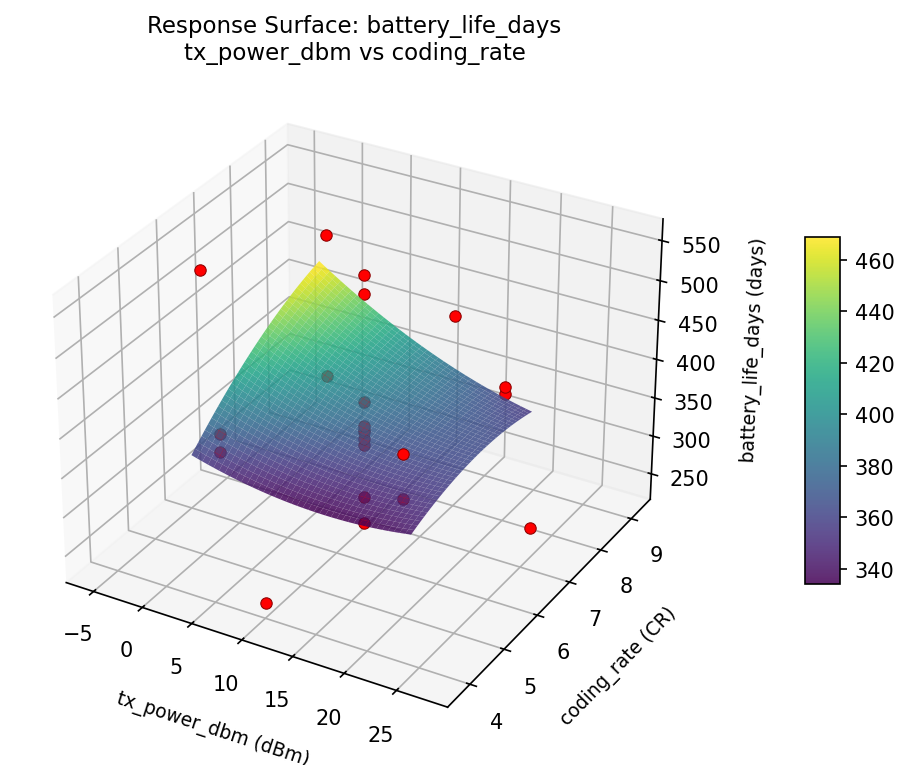
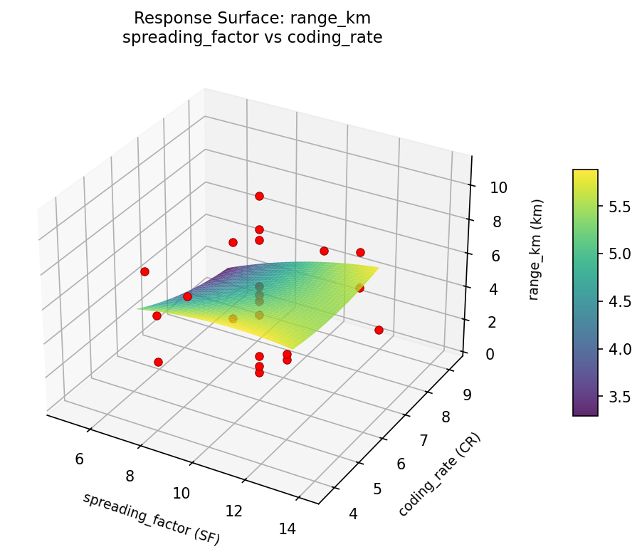
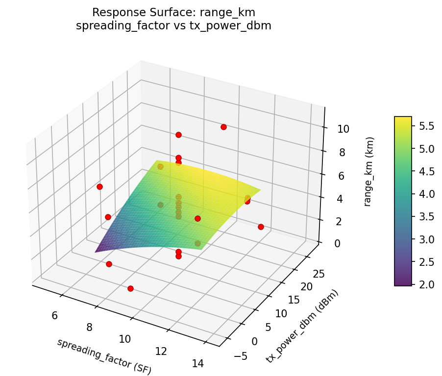
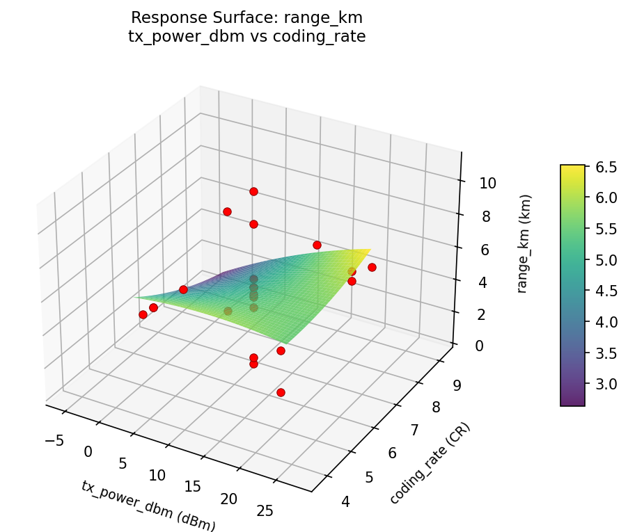
Response Surface Plots
3D surfaces fitted with quadratic RSM. Red dots are observed data points.
battery life days spreading factor vs coding rate
battery life days spreading factor vs tx power dbm
battery life days tx power dbm vs coding rate
range km spreading factor vs coding rate
range km spreading factor vs tx power dbm
range km tx power dbm vs coding rate
Multi-Objective Optimization
When responses compete, Derringer–Suich desirability finds the best compromise.
Each response is scaled to a 0–1 desirability, then combined via a weighted geometric mean.
Overall Desirability
D = 0.4770
Per-Response Desirability
| Response | Weight | Desirability | Predicted | Dir |
|---|
range_km |
1.5 |
|
6.90 0.6049 6.90 km |
↑ |
battery_life_days |
1.0 |
|
339.00 0.3341 339.00 days |
↑ |
Recommended Settings
| Factor | Value |
|---|
spreading_factor | 14.0644 SF |
tx_power_dbm | 11 dBm |
coding_rate | 6.5 CR |
Source: from observed run #17
Trade-off Summary
Sacrifice = how much worse than single-objective best.
| Response | Predicted | Best Observed | Sacrifice |
|---|
battery_life_days | 339.00 | 554.00 | +215.00 |
Top 3 Runs by Desirability
| Run | D | Factor Settings |
|---|
| #22 | 0.4675 | spreading_factor=7, tx_power_dbm=2, coding_rate=5 |
| #4 | 0.4505 | spreading_factor=12, tx_power_dbm=20, coding_rate=5 |
Model Quality
| Response | R² | Type |
|---|
battery_life_days | 0.1100 | linear |
Full Multi-Objective Output
============================================================
MULTI-OBJECTIVE OPTIMIZATION
Method: Derringer-Suich Desirability Function
============================================================
Overall desirability: D = 0.4770
Response Weight Desirability Predicted Direction
---------------------------------------------------------------------
range_km 1.5 0.6049 6.90 km ↑
battery_life_days 1.0 0.3341 339.00 days ↑
Recommended settings:
spreading_factor = 14.0644 SF
tx_power_dbm = 11 dBm
coding_rate = 6.5 CR
(from observed run #17)
Trade-off summary:
range_km: 6.90 (best observed: 10.90, sacrifice: +4.00)
battery_life_days: 339.00 (best observed: 554.00, sacrifice: +215.00)
Model quality:
range_km: R² = 0.1712 (linear)
battery_life_days: R² = 0.1100 (linear)
Top 3 observed runs by overall desirability:
1. Run #17 (D=0.4770): spreading_factor=14.0644, tx_power_dbm=11, coding_rate=6.5
2. Run #22 (D=0.4675): spreading_factor=7, tx_power_dbm=2, coding_rate=5
3. Run #4 (D=0.4505): spreading_factor=12, tx_power_dbm=20, coding_rate=5
Full Analysis Output
=== Main Effects: range_km ===
Factor Effect Std Error % Contribution
--------------------------------------------------------------
tx_power_dbm 6.2500 0.5851 51.7%
coding_rate 5.2500 0.5851 43.4%
spreading_factor 0.5833 0.5851 4.8%
=== ANOVA Table: range_km ===
Source DF SS MS F p-value
-----------------------------------------------------------------------------
spreading_factor 4 1.2715 0.3179 0.035 0.9972
tx_power_dbm 4 40.4840 10.1210 1.113 0.4080
coding_rate 4 33.4807 8.3702 0.920 0.4929
Lack of Fit 2 19.2432 9.6216 1.058 0.3968
Pure Error 7 63.6588 9.0941
Error 9 82.9020 9.0941
Total 21 158.1382 7.5304
=== Summary Statistics: range_km ===
spreading_factor:
Level N Mean Std Min Max
------------------------------------------------------------
12 4 5.0500 3.3392 0.9000 9.0000
14.0644 1 5.2000 0.0000 5.2000 5.2000
4.93565 1 4.8000 0.0000 4.8000 4.8000
7 4 5.2750 1.2258 4.0000 6.9000
9.5 12 4.6917 3.2878 0.5000 10.9000
tx_power_dbm:
Level N Mean Std Min Max
------------------------------------------------------------
-5.43168 1 4.8000 0.0000 4.8000 4.8000
11 12 5.0833 3.0114 0.7000 10.9000
2 4 6.7500 1.6340 5.4000 9.0000
20 4 3.5750 1.8154 0.9000 4.8000
27.4317 1 0.5000 0.0000 0.5000 0.5000
coding_rate:
Level N Mean Std Min Max
------------------------------------------------------------
3.76139 1 2.0000 0.0000 2.0000 2.0000
5 4 5.9500 2.0616 4.6000 9.0000
6.5 12 5.3000 2.8851 0.5000 10.9000
8 4 4.3750 2.6043 0.9000 6.9000
9.23861 1 0.7000 0.0000 0.7000 0.7000
=== Main Effects: battery_life_days ===
Factor Effect Std Error % Contribution
--------------------------------------------------------------
tx_power_dbm 220.5000 18.1371 51.2%
coding_rate 169.5000 18.1371 39.4%
spreading_factor 40.5000 18.1371 9.4%
=== ANOVA Table: battery_life_days ===
Source DF SS MS F p-value
-----------------------------------------------------------------------------
spreading_factor 4 2503.5909 625.8977 0.084 0.9852
tx_power_dbm 4 46473.5909 11618.3977 1.564 0.2646
coding_rate 4 28375.6742 7093.9186 0.955 0.4764
Lack of Fit 2 22630.8598 11315.4299 1.523 0.2823
Pure Error 7 51992.8750 7427.5536
Error 9 74623.7348 7427.5536
Total 21 151976.5909 7236.9805
=== Summary Statistics: battery_life_days ===
spreading_factor:
Level N Mean Std Min Max
------------------------------------------------------------
12 4 376.0000 109.8271 273.0000 531.0000
14.0644 1 357.0000 0.0000 357.0000 357.0000
4.93565 1 348.0000 0.0000 348.0000 348.0000
7 4 377.0000 25.9872 339.0000 396.0000
9.5 12 388.5000 100.5715 239.0000 554.0000
tx_power_dbm:
Level N Mean Std Min Max
------------------------------------------------------------
-5.43168 1 379.0000 0.0000 379.0000 379.0000
11 12 369.5000 86.3823 239.0000 521.0000
2 4 333.5000 45.0370 273.0000 382.0000
20 4 419.5000 76.0197 360.0000 531.0000
27.4317 1 554.0000 0.0000 554.0000 554.0000
coding_rate:
Level N Mean Std Min Max
------------------------------------------------------------
3.76139 1 423.0000 0.0000 423.0000 423.0000
5 4 351.5000 53.9290 273.0000 391.0000
6.5 12 368.5833 90.6476 239.0000 554.0000
8 4 401.5000 90.3493 339.0000 531.0000
9.23861 1 521.0000 0.0000 521.0000 521.0000
Optimization Recommendations
=== Optimization: range_km ===
Direction: maximize
Best observed run: #18
spreading_factor = 9.5
tx_power_dbm = 11
coding_rate = 3.76139
Value: 10.9
RSM Model (linear, R² = 0.0394, Adj R² = -0.1207):
Coefficients:
intercept +4.8909
spreading_factor -0.6239
tx_power_dbm -0.1236
coding_rate -0.1431
RSM Model (quadratic, R² = 0.6301, Adj R² = 0.3526):
Coefficients:
intercept +5.5449
spreading_factor -0.6239
tx_power_dbm -0.1235
coding_rate -0.1431
spreading_factor*tx_power_dbm +0.6625
spreading_factor*coding_rate -1.1375
tx_power_dbm*coding_rate +1.2875
spreading_factor^2 -1.1120
tx_power_dbm^2 -0.8870
coding_rate^2 +1.0180
Curvature analysis:
spreading_factor coef=-1.1120 concave (has a maximum)
coding_rate coef=+1.0180 convex (has a minimum)
tx_power_dbm coef=-0.8870 concave (has a maximum)
Notable interactions:
tx_power_dbm*coding_rate coef=+1.2875 (synergistic)
spreading_factor*coding_rate coef=-1.1375 (antagonistic)
spreading_factor*tx_power_dbm coef=+0.6625 (synergistic)
Predicted optimum (from quadratic model, at observed points):
spreading_factor = 9.5
tx_power_dbm = 11
coding_rate = 3.76139
Predicted value: 9.1996
Surface optimum (via L-BFGS-B, quadratic model):
spreading_factor = 9.48309
tx_power_dbm = 3.81841
coding_rate = 5
Predicted value: 7.2672
Model quality: Moderate fit — use predictions directionally, not precisely.
Factor importance:
1. coding_rate (effect: 7.3, contribution: 44.0%)
2. spreading_factor (effect: 5.4, contribution: 32.9%)
3. tx_power_dbm (effect: 3.8, contribution: 23.1%)
=== Optimization: battery_life_days ===
Direction: maximize
Best observed run: #6
spreading_factor = 14.0644
tx_power_dbm = 11
coding_rate = 6.5
Value: 554.0
RSM Model (linear, R² = 0.0793, Adj R² = -0.0742):
Coefficients:
intercept +380.8636
spreading_factor +28.4777
tx_power_dbm -0.7955
coding_rate +3.1302
RSM Model (quadratic, R² = 0.6515, Adj R² = 0.3902):
Coefficients:
intercept +362.8899
spreading_factor +28.4772
tx_power_dbm -0.7955
coding_rate +3.1302
spreading_factor*tx_power_dbm -37.5000
spreading_factor*coding_rate +39.5000
tx_power_dbm*coding_rate -37.7500
spreading_factor^2 +35.4866
tx_power_dbm^2 +19.1369
coding_rate^2 -27.6631
Curvature analysis:
spreading_factor coef=+35.4866 convex (has a minimum)
coding_rate coef=-27.6631 concave (has a maximum)
tx_power_dbm coef=+19.1369 convex (has a minimum)
Notable interactions:
spreading_factor*coding_rate coef=+39.5000 (synergistic)
tx_power_dbm*coding_rate coef=-37.7500 (antagonistic)
spreading_factor*tx_power_dbm coef=-37.5000 (antagonistic)
Predicted optimum (from quadratic model, at observed points):
spreading_factor = 12
tx_power_dbm = 2
coding_rate = 8
Predicted value: 537.0032
Surface optimum (via L-BFGS-B, quadratic model):
spreading_factor = 12
tx_power_dbm = 2
coding_rate = 8
Predicted value: 537.0032
Model quality: Moderate fit — use predictions directionally, not precisely.
Factor importance:
1. spreading_factor (effect: 205.8, contribution: 46.1%)
2. coding_rate (effect: 175.2, contribution: 39.2%)
3. tx_power_dbm (effect: 65.8, contribution: 14.7%)