Distributed Deep Learning

Summary

This experiment investigates distributed deep learning scaling. Optimize multi-GPU distributed training configuration for ResNet-50 on ImageNet.

The design varies 3 factors: gpu count (GPUs), ranging from 8 to 64, batch per gpu (images), ranging from 32 to 256, and gradient compression (%), ranging from 0 to 90. The goal is to optimize 2 responses: images per sec (img/s) (maximize) and scaling efficiency (%) (maximize).

A Box-Behnken design was chosen because it efficiently fits quadratic models with 3 continuous factors while avoiding extreme corner combinations — requiring only 15 runs instead of the 8 needed for a full factorial at two levels.

Quadratic response surface models were fitted to capture potential curvature and factor interactions. The RSM contour plots below visualize how pairs of factors jointly affect each response.

Key Findings

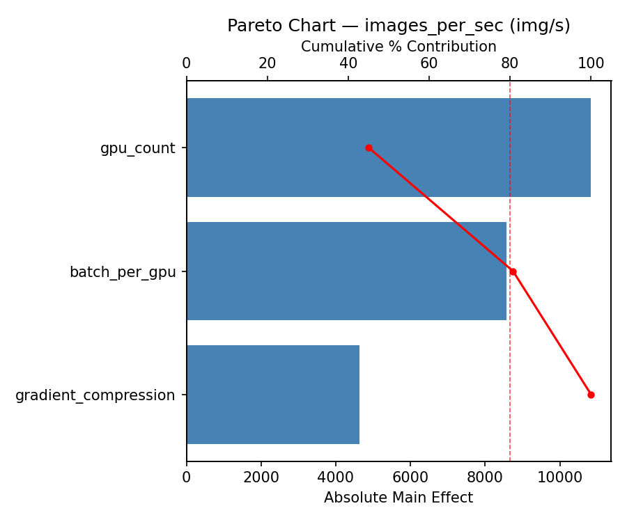
For images per sec, the most influential factors were batch per gpu (42.1%), gradient compression (39.2%), gpu count (18.7%). The best observed value was 27276.1 (at gpu count = 64, batch per gpu = 256, gradient compression = 45).

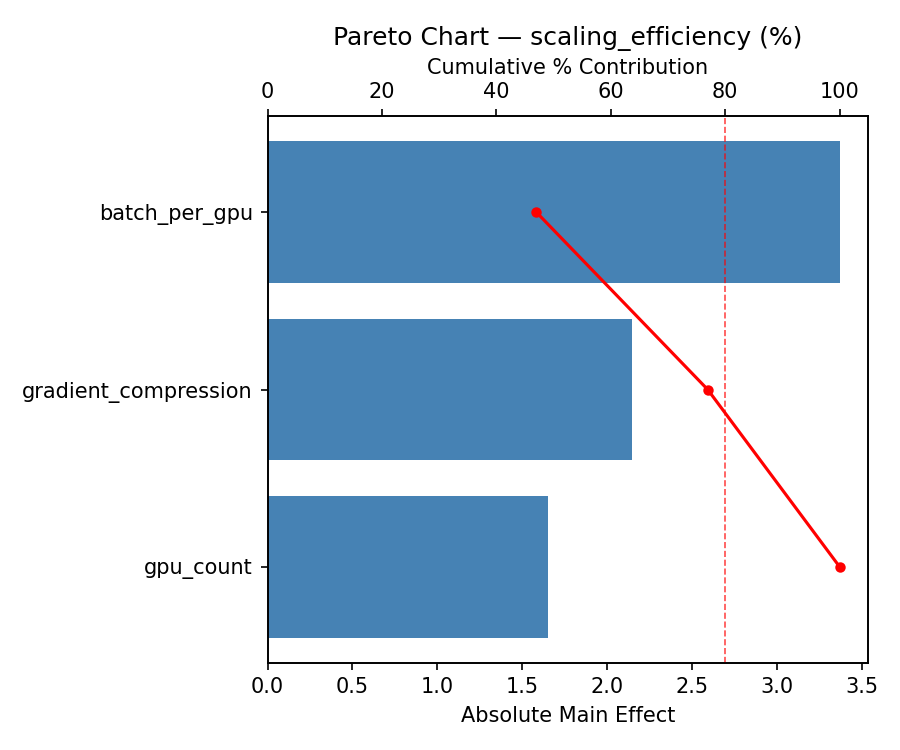
For scaling efficiency, the most influential factors were gradient compression (45.2%), batch per gpu (36.3%), gpu count (18.5%). The best observed value was 99.0 (at gpu count = 8, batch per gpu = 256, gradient compression = 45).

Recommended Next Steps

Run confirmation experiments at the predicted optimal settings to validate the model.
Consider whether any fixed factors should be varied in a future study.

Experimental Setup

Factors

Factor	Levels	Type	Unit
`gpu_count`	8, 64	continuous	GPUs
`batch_per_gpu`	32, 256	continuous	images
`gradient_compression`	0, 90	continuous	%

Fixed: none

Responses

Response	Direction	Unit
`images_per_sec`	↑ maximize	img/s
`scaling_efficiency`	↑ maximize	%

Experimental Matrix

The Box-Behnken Design produces 15 runs. Each row is one experiment with specific factor settings.

Run	`gpu_count`	`batch_per_gpu`	`gradient_compression`
1	36	32	0
2	36	144	45
3	64	144	90
4	64	144	0
5	36	144	45
6	36	144	45
7	8	144	90
8	64	32	45
9	36	32	90
10	64	256	45
11	8	144	0
12	36	256	90
13	8	32	45
14	8	256	45
15	36	256	0

How to Run

terminal
$ doe info --config use_cases/15_distributed_training/config.json
$ doe generate --config use_cases/15_distributed_training/config.json --output results/run.sh --seed 42
$ bash results/run.sh
$ doe analyze --config use_cases/15_distributed_training/config.json
$ doe optimize --config use_cases/15_distributed_training/config.json
$ doe report --config use_cases/15_distributed_training/config.json --output report.html

Analysis Results

Generated from actual experiment runs.

Response: images_per_sec

Pareto Chart

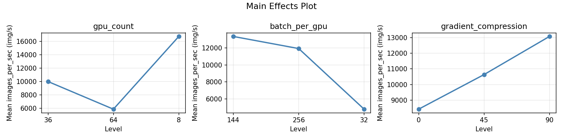
Main Effects Plot

Response: scaling_efficiency

Pareto Chart

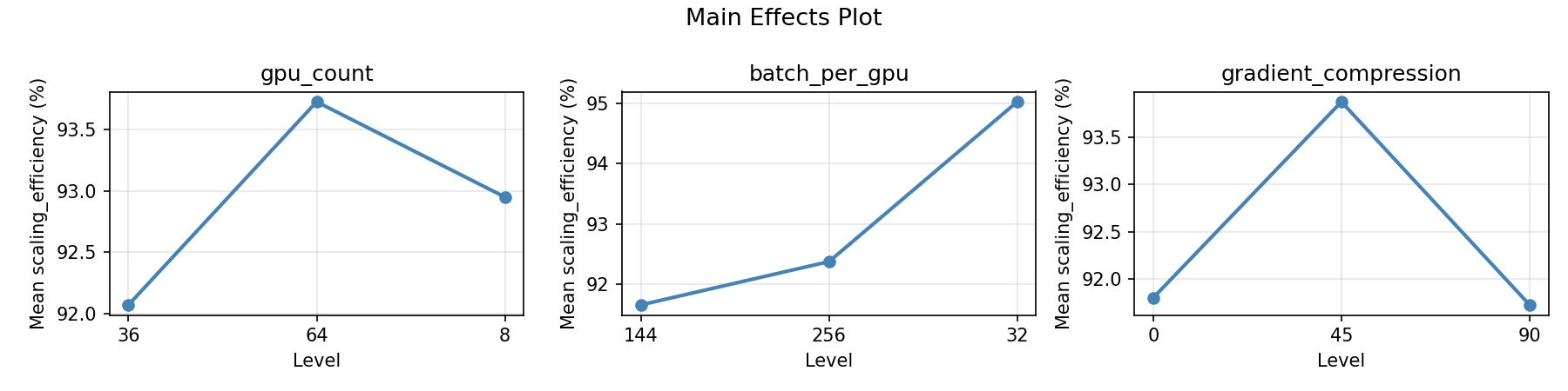
Main Effects Plot

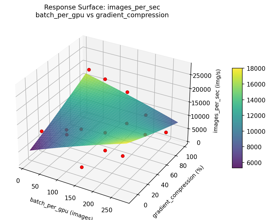
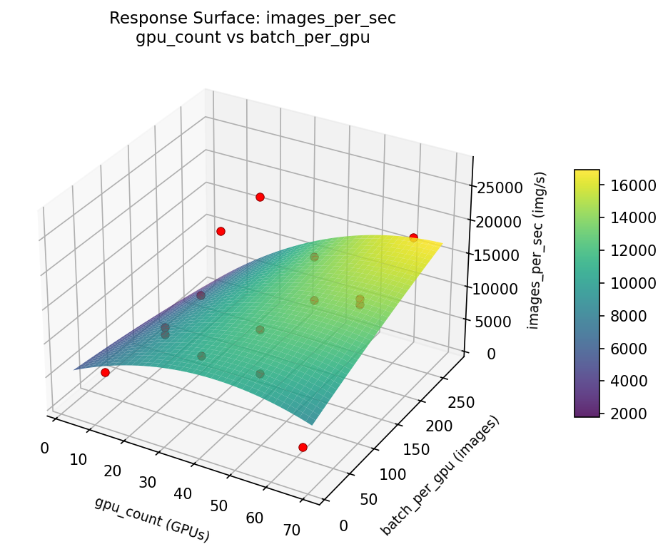
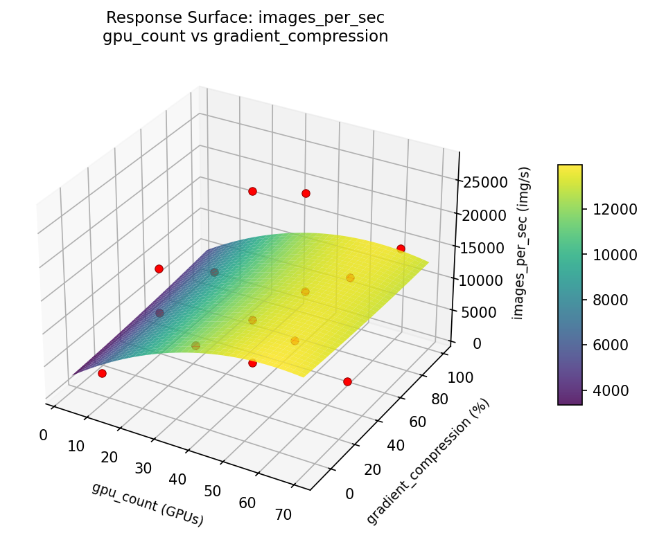
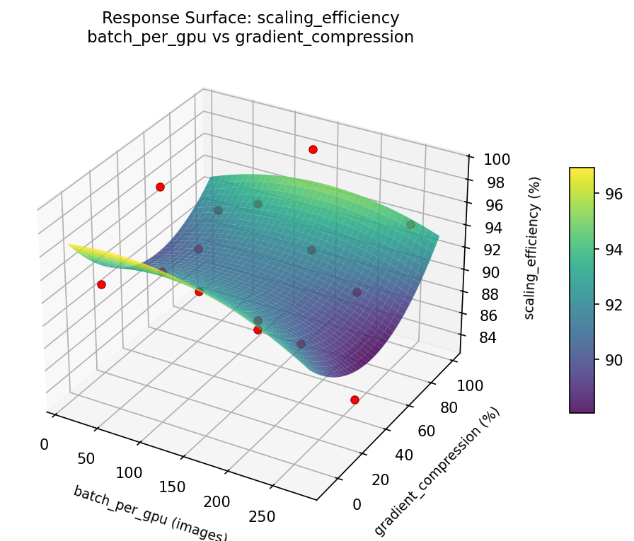
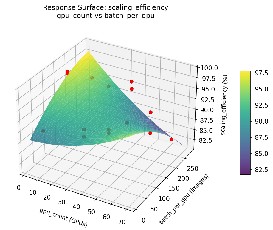
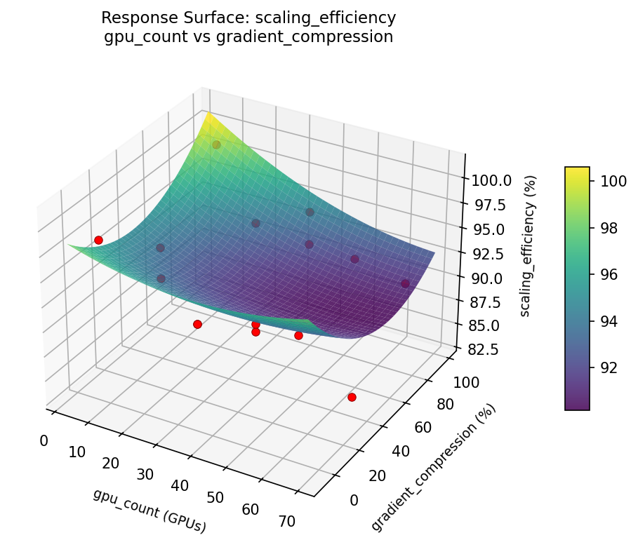
Response Surface Plots

3D surfaces fitted with quadratic RSM. Red dots are observed data points.

📊

How to Read These Surfaces

Each plot shows predicted response (vertical axis) across two factors while other factors are held at center. Red dots are actual experimental observations.

Flat surface — these two factors have little effect on the response.
Tilted plane — strong linear effect; moving along one axis consistently changes the response.
Curved/domed surface — quadratic curvature; there is an optimum somewhere in the middle.
Saddle shape — significant interaction; the best setting of one factor depends on the other.
Red dots far from surface — poor model fit in that region; be cautious about predictions there.

images_per_sec (img/s) — R² = 0.831, Adj R² = 0.526
Moderate fit — surface shows general trends but some noise remains.
Curvature detected in batch_per_gpu, gradient_compression — look for a peak or valley in the surface.
Strongest linear driver: batch_per_gpu (increases images_per_sec).
Notable interaction: gpu_count × batch_per_gpu — the effect of one depends on the level of the other. Look for a twisted surface.

scaling_efficiency (%) — R² = 0.627, Adj R² = -0.045
Moderate fit — surface shows general trends but some noise remains.
Curvature detected in gradient_compression, gpu_count — look for a peak or valley in the surface.
Strongest linear driver: batch_per_gpu (decreases scaling_efficiency).
Notable interaction: gpu_count × batch_per_gpu — the effect of one depends on the level of the other. Look for a twisted surface.

images: per sec batch per gpu vs gradient compression

images: per sec gpu count vs batch per gpu

images: per sec gpu count vs gradient compression

scaling: efficiency batch per gpu vs gradient compression

scaling: efficiency gpu count vs batch per gpu

scaling: efficiency gpu count vs gradient compression

Full Analysis Output

doe analyze
=== Main Effects: images_per_sec ===
Factor                   Effect    Std Error   % Contribution
--------------------------------------------------------------
gpu_count             9143.9500    1997.6298            42.1%
gradient_compression  6382.5000    1997.6298            29.4%
batch_per_gpu         6215.2000    1997.6298            28.6%

=== Summary Statistics: images_per_sec ===

gpu_count:
  Level               N       Mean        Std        Min        Max
  ------------------------------------------------------------
  36                  7  9785.4286  7214.6845  1100.5000 20235.7000
  64                  4  6920.5750  3516.3765  3806.9000 11499.3000
  8                   4 16064.5250 10173.5266  2693.1000 27276.1000

batch_per_gpu:
  Level               N       Mean        Std        Min        Max
  ------------------------------------------------------------
  144                 7 10633.8571  9817.8742  1100.5000 27276.1000
  256                 4  7642.5750  7297.1113  2723.4000 18500.0000
  32                  4 13857.7750  2745.5949 11499.3000 16643.6000

gradient_compression:
  Level               N       Mean        Std        Min        Max
  ------------------------------------------------------------
  0                   4  6466.7500  6804.3168  2693.1000 16643.6000
  45                  7 11882.0571  7060.7804  1100.5000 20235.7000
  90                  4 12849.2500 10000.7841  4796.2000 27276.1000

=== Main Effects: scaling_efficiency ===
Factor                   Effect    Std Error   % Contribution
--------------------------------------------------------------
gradient_compression     6.7750       1.1818            48.7%
gpu_count                5.3250       1.1818            38.3%
batch_per_gpu            1.8143       1.1818            13.0%

=== Summary Statistics: scaling_efficiency ===

gpu_count:
  Level               N       Mean        Std        Min        Max
  ------------------------------------------------------------
  36                  7    94.8000     2.7080    91.3000    98.5000
  64                  4    92.4250     4.8624    87.9000    99.0000
  8                   4    89.4750     5.9337    83.4000    97.4000

batch_per_gpu:
  Level               N       Mean        Std        Min        Max
  ------------------------------------------------------------
  144                 7    93.4143     4.9144    87.1000    99.0000
  256                 4    91.6000     6.5243    83.4000    98.5000
  32                  4    92.7250     2.0255    90.0000    94.9000

gradient_compression:
  Level               N       Mean        Std        Min        Max
  ------------------------------------------------------------
  0                   4    97.4500     1.8267    94.9000    99.0000
  45                  7    91.2429     4.4669    83.4000    98.2000
  90                  4    90.6750     3.7456    87.1000    94.7000

Optimization Recommendations

doe optimize
=== Optimization: images_per_sec ===
Direction: maximize

Best observed run: #10
  gpu_count = 64
  batch_per_gpu = 256
  gradient_compression = 45
  Value: 27276.1

RSM Model (linear, R² = 0.05):
  Coefficients:
    intercept:  +10695.8933
    gpu_count:  +1634.1250
    batch_per_gpu:  +1714.1500
    gradient_compression:  -369.2250
  Predicted optimum:
    gpu_count = 64
    batch_per_gpu = 256
    gradient_compression = 45
    Predicted value: 14044.1683

Factor importance:
  1. batch_per_gpu  (effect: 6246.3, contribution: 44.0%)
  2. gradient_compression  (effect: 4686.9, contribution: 33.0%)
  3. gpu_count  (effect: 3268.3, contribution: 23.0%)

=== Optimization: scaling_efficiency ===
Direction: maximize

Best observed run: #14
  gpu_count = 36
  batch_per_gpu = 144
  gradient_compression = 45
  Value: 99.0

RSM Model (linear, R² = 0.02):
  Coefficients:
    intercept:  +92.7467
    gpu_count:  +0.8125
    batch_per_gpu:  -0.2125
    gradient_compression:  +0.1000
  Predicted optimum:
    gpu_count = 64
    batch_per_gpu = 32
    gradient_compression = 45
    Predicted value: 93.7717

Factor importance:
  1. batch_per_gpu  (effect: 5.1, contribution: 66.5%)
  2. gpu_count  (effect: 1.6, contribution: 21.2%)
  3. gradient_compression  (effect: 1.0, contribution: 12.4%)

Multi-Objective Optimization

When responses compete, Derringer–Suich desirability finds the best compromise. Each response is scaled to a 0–1 desirability, then combined via a weighted geometric mean.

Overall Desirability

D = 0.6343

Per-Response Desirability

Response	Weight	Desirability	Predicted	Dir
`images_per_sec`	1.5	0.5853	16643.60 0.5853 16643.60 img/s	↑
`scaling_efficiency`	1.0	0.7156	94.90 0.7156 94.90 %	↑

Recommended Settings

Factor	Value
`gpu_count`	8 GPUs
`batch_per_gpu`	144 images
`gradient_compression`	90 %

Source: from observed run #12

Trade-off Summary

Sacrifice = how much worse than single-objective best.

Response	Predicted	Best Observed	Sacrifice
`scaling_efficiency`	94.90	99.00	+4.10

Top 3 Runs by Desirability

Run	D	Factor Settings
#3	0.6200	gpu_count=36, batch_per_gpu=144, gradient_compression=45
#10	0.5683	gpu_count=64, batch_per_gpu=144, gradient_compression=90

Model Quality

Response	R²	Type
`scaling_efficiency`	0.1230	linear

Full Multi-Objective Output

doe optimize --multi
============================================================
MULTI-OBJECTIVE OPTIMIZATION
Method: Derringer-Suich Desirability Function
============================================================

Overall desirability: D = 0.6343

Response                  Weight Desirability    Predicted  Direction
---------------------------------------------------------------------
images_per_sec               1.5       0.5853    16643.60 img/s   ↑
scaling_efficiency           1.0       0.7156       94.90 %   ↑

Recommended settings:
  gpu_count = 8 GPUs
  batch_per_gpu = 144 images
  gradient_compression = 90 %
  (from observed run #12)

Trade-off summary:
  images_per_sec: 16643.60 (best observed: 27276.10, sacrifice: +10632.50)
  scaling_efficiency: 94.90 (best observed: 99.00, sacrifice: +4.10)

Model quality:
  images_per_sec: R² = 0.1313 (linear)
  scaling_efficiency: R² = 0.1230 (linear)

Top 3 observed runs by overall desirability:
  1. Run #12 (D=0.6343): gpu_count=8, batch_per_gpu=144, gradient_compression=90
  2. Run #3 (D=0.6200): gpu_count=36, batch_per_gpu=144, gradient_compression=45
  3. Run #10 (D=0.5683): gpu_count=64, batch_per_gpu=144, gradient_compression=90

Run	`gpu_count`	`batch_per_gpu`	`gradient_compression`
1	36	32	0
2	36	144	45
3	64	144	90
4	64	144	0
5	36	144	45
6	36	144	45
7	8	144	90
8	64	32	45
9	36	32	90
10	64	256	45
11	8	144	0
12	36	256	90
13	8	32	45
14	8	256	45
15	36	256	0

Run	`gpu_count`	`batch_per_gpu`	`gradient_compression`
1	36	32	0
2	36	144	45
3	64	144	90
4	64	144	0
5	36	144	45
6	36	144	45
7	8	144	90
8	64	32	45
9	36	32	90
10	64	256	45
11	8	144	0
12	36	256	90
13	8	32	45
14	8	256	45
15	36	256	0

Run	`gpu_count`	`batch_per_gpu`	`gradient_compression`
1	36	32	0
2	36	144	45
3	64	144	90
4	64	144	0
5	36	144	45
6	36	144	45
7	8	144	90
8	64	32	45
9	36	32	90
10	64	256	45
11	8	144	0
12	36	256	90
13	8	32	45
14	8	256	45
15	36	256	0